Bob Shiller defines “narrative economics” as the study of “how narrative contagion affects economic events”. This research program focuses on two things: “(1) the word-of-mouth contagion of ideas in the form of stories and (2) the efforts that people make to generate new contagious stories or to make stories more contagious.” In other words, if you could somehow get people to stop telling each other tall tales, then stock prices, GDP, interest rates, housing sales, etc would be different.
I’m a huge fan of this work. And even the most ardent critics of narrative economics still appreciate the power of a good narrative. For example, like all economics papers, the Campbell-Cochrane habit-formation paper has an introduction. The introduction gives an intuitive explanation of how the paper works using evocative language. The paper is called By Force of Habit for god’s sake. If that isn’t an effort to make the paper’s story more contagious, I don’t know what is.
But many researchers feel that narrative economics (in its current form) is less than scientific. And I think there’s something to these claims. Narrative economics says that economic outcomes are different because of the fact that people tell each other stories and embellish these stories in the process. But there are no specific parameters corresponding to these two tendencies in any economic model. Put differently, There’s no “narrative” in models of “narrative economics”. Whether or not a paper gets classified as a narrative-based model often comes down to how it’s written. This makes it hard to analyze how tall tales affect economic outcomes. What would the counterfactual world without the contagious narratives look like?
Compare and contrast this state of affairs how other economic forces get modeled. For example, the Campbell-Cochrane habit-formation paper allows risk aversion to vary over time. We know this because we can directly point to this parameter in the model. And, as a result, we can imagine a world where risk aversion is no longer allowed to vary over time. It’s not clear how to do the same thing in narrative-based models. There’s no parameter that corresponds to the story-telling instinct.
To place narrative economics on firm footing, we need some way of toggling on and off peoples’ tendency to tell tall tales in our models. There needs to be a narrative module in our models. That way, we can analyze the effect of this module on things like stock prices, GDP, interest rates, housing sales, etc. This post highlights two problems with current narrative-based models that make it difficult to accomplish this goal. Then, I conclude by suggesting a way to put the “narrative” into models of narrative economics.
Narratives aren’t the only kind of epidemic
When Shiller talks and writes about narrative economics, he plays up the importance of how stories go “viral”. The reason why narratives have the power to affect economic outcomes is that they can spread contagiously from person to person via word of mouth like a meme or viruse. Shiller has been a strong proponent of using epidemiological models to study financial markets. I’m a huge fan of this idea! I’ve even got a paper which takes this exact approach. Epidemiological models can tell us a lot about how trader interactions affect market outcomes, leading to things like booms and busts.
That being said, it’s important to emphasize that there is no “narrative” in epidemiological models. In these models, something is exchanged when two agents interact with one another. That something could be a virus, a story, or an Egg McMuffin recipe. Anything that these models say about narratives must also apply to a virus or a delicious new way to start your day. Epidemiological models are models of interacting agents not models of what happens when agents interact. Social finance and narrative economics are distinct fields.
Suppose there are  people, of which,
  are currently sick. The remaining
  people are healthy. Each instant, a sick person encounters a healthy person with probability
  . And, when that happens, the healthy person becomes sick at a rate of
  per interaction. Otherwise, sick people recover with probability
  each instant. This implies that the total population of sick people will evolve as
(1) ![\begin{equation*} \mathrm{d}S = \underset{\text{contract disease}}{[\beta \cdot (H/N) \cdot S] \cdot \mathrm{d}t} - \underset{\text{get healthy}}{[\gamma \cdot S] \cdot \mathrm{d}t} \end{equation*}](https://alexchinco.com/wp-content/ql-cache/quicklatex.com-85201af680984c8abd60b6ffafc58453_l3.svg "Rendered by QuickLaTeX.com")
Flipping the logic around then says that the population of healthy people must evolve according to:
(2) ![\begin{equation*} \mathrm{d}H = \underset{\text{get healthy}}{[\gamma \cdot S] \cdot \mathrm{d}t} - \underset{\text{contract disease}}{[\beta \cdot (S/N) \cdot H] \cdot \mathrm{d}t} \end{equation*}](https://alexchinco.com/wp-content/ql-cache/quicklatex.com-db4335a5882bfa3581439f721e9c541a_l3.svg "Rendered by QuickLaTeX.com")
Notice that there is no biology in this model. There’s nothing specific to structure of viruses or the life cycle of bacteria. There are just two interacting populations. These could be sick and healthy people. Or they could be excited speculators and rational investors. Epidemiological models can capture how an economic narrative spreads through a population. But they can tell us nothing about what an economic narrative actually is. This is a non-starter. We want to be able to plug the narrative module (whatever that happens to be) into an epidemiological model. But a narrative is different from how it spreads.
The tell-tale signs of people telling tall tales
Right now, economists mainly think in terms of models where investors solve forward-looking constrained optimization problems. Narrative economics argues that it’s valuable to think about narratives and models rather than just models. If this is true, then the story-telling instinct must be able to explain phenomenon that the existing paradigm can’t. Narratives must be more than just bad explanations. They must be something that is fundamentally outside the currently modeling paradigm. Otherwise, it won’t be possible to distinguish the implications of the narrative from the implications of a fine-tuned economic model.
Here’s what I mean. There are several recent papers (e.g., see here and here) that study narratives by incorporating ideas from the causal-inference literature. These papers model narratives using directed acyclical graphs (DAGs). If you have an underlying structural-equation model for the economy, then you can represent this model’s causal implications using a DAG in a way that is largely independent of the magnitudes of the parameter values involved. All that matters is the zero vs nonzero distinction.
Causal relationships without nitty-gritty parameter estimates… this might at first seem like a promising way of modeling narratives. But here’s the thing: anything that can be captured by a DAG can also be written down as a standard economic model. So, if you model narratives using DAGs, it can never be clear which is the real driver—the narrative or the underlying model.
To illustrate, suppose that the Campbell-Cochrane habit-formation model were strictly true. Suppose that the model in that paper was actually the data-generating process for observed asset-prices in the real world. In this fictitious scenario, further suppose that whenever you ask traders, they talk about the world in exactly the way that Campbell and Cochrane do in their introduction. In this set up, traders’ would have a clear narrative about what was going on in the market, and this narrative would fit perfectly into a DAG. But the narrative would not be responsible for the observed market data. If you didn’t ask traders about what they were doing, all economic outcomes would be the exact same.
DAGs capture the component of narratives that could be incorporated into well-posed model. If it’s important to consider narratives in addition to standard economic models, then their contribution must come from something that cannot be captured by simply adding a new variable to a DAG. Narrative economics must represent more than just throwing away some of the information in a model.
Narratives determine how people construe events
Narrative economics says that economic outcomes are different because people tell each other stories that get exaggerated with each retelling. To test this claim, we want some way of adding a narrative to an existing economic model. Then, we can flip the story-telling instinct on and off in the model and examine the consequences.
Whatever this narrative module looks like, it won’t be tied to epidemiological models. These models aren’t specific to narratives. They’re called “epidemiological models” for a reason. What’s more, if we want to distinguish narrative economics from the existing model-based paradigm, then a narrative must be more than just a new variable or parameter. Otherwise, it would be easy to achieve the same results using a standard model. If all you do is show that prices tend to go up with there are more positive words in the Wall Street Journal, it’s easy to gin up alternative stories that don’t involve investors tell each other good stories.
We can’t define a narrative by studying epidemiological models. And we can’t associate a narrative with a single new variable or parameter? Where does that leave us?
In his 2013 Nobel Prize lecture, Bob Shiller urged economists to incorporate more ideas from psychology, sociology, and other fields. And I think this is exactly the right way to go. But, rather than turning to epidemiology, let’s look at the subfield of psychology that studies the interface between language and the mind—namely, cognitive linguistics. We want to identify the economic effects of conveying information between people via the medium of story. It stands to reason that stories might be stored differently by the brain relative to statistics, song, interpretive dance, divine proclamation, etc.
Cognitive linguistics tells us that stories affect how people “construe events” being related to one another. For example, the force dynamics paradigm says that letting something be is not the same as pushing on it with zero force even though these two situations are identical according to every physics textbook. The narrative module we are looking for should tell us when to construe the same events in different ways.
Here’s another example. Suppose there are  people with a deadly disease and doctors are asked to choose between two treatments. Treatment A results in
  deaths. Under treatment B there is a
  chance that no one will die but a
  chance that all people will die. The narrative should explain whether doctors frame this famous choice as “(treatment A saves
  and treatment B kills everyone of the time)” or as “(treatment A kills people and treatment B saves everyone of the time)”.
There is direct evidence that human brains reason about stories using something like the force dynamics paradigm (e.g., see studies like this one). So we are not talking about layering on a “narrative interpretation” to a model as is the case with epidemiological models. And, if a story can change the *relationships among entire collections of variables*, it’s not easy to account for its predictions using a single existing model. Because its effects are non-local, you would need an entirely new model for each construal of events. Turning off the narrative module would be akin to steadfastly adhering to only one model. A narrative module should account for the way that people pick and choose which model to apply at different points in time. That’s my guess about how to model the “narrative” in “narrative economics”.
 stocks. Next period, the
  th stock will realize a relative return of
 ![R[n] \in \{-1, \, +\!1 \}](https://alexchinco.com/wp-content/ql-cache/quicklatex.com-2445a8f41c0f5dc3e2496e7e7ed5165a_l3.svg "Rendered by QuickLaTeX.com") . If the stock’s return is above average, then
. If the stock’s return is above average, then ![R[n] = +1](https://alexchinco.com/wp-content/ql-cache/quicklatex.com-7d6328012f9cfff5b740894cf6f97e3b_l3.svg "Rendered by QuickLaTeX.com") . If its return is below average, then
. If its return is below average, then ![R[n] = -1](https://alexchinco.com/wp-content/ql-cache/quicklatex.com-63a90fd64854e9969f467779b22f0406_l3.svg "Rendered by QuickLaTeX.com") . You could add finer gradations—positive, zero, and negative—very positive, positive, zero, negative, and very negative—and so on. But for now let’s just study a binary world for simplicity’s sake.
. You could add finer gradations—positive, zero, and negative—very positive, positive, zero, negative, and very negative—and so on. But for now let’s just study a binary world for simplicity’s sake. characteristics. Let
 ![X_k[n]](https://alexchinco.com/wp-content/ql-cache/quicklatex.com-331a111b6b3ef21e53d55815c04cef77_l3.svg "Rendered by QuickLaTeX.com") denote the value of the
denote the value of the  th characteristic for the
 ![\boldsymbol{X}[n] = \{ X_k[n] \}_{k=1}^K](https://alexchinco.com/wp-content/ql-cache/quicklatex.com-80909f52ccdfa8510fe975fbe4f5f072_l3.svg "Rendered by QuickLaTeX.com") denote a vector containing the values of all
denote a vector containing the values of all  characteristics for the
  rather than
 ![(R[n], \, \boldsymbol{X}[n])](https://alexchinco.com/wp-content/ql-cache/quicklatex.com-c4e25320754d485361cab291dd40e31f_l3.svg "Rendered by QuickLaTeX.com") .
.![\{ R[n] \}_{n=1}^N](https://alexchinco.com/wp-content/ql-cache/quicklatex.com-08a6bd3c48b9339c1f28efb433a058f7_l3.svg "Rendered by QuickLaTeX.com") . Your goal is to find some function,
. Your goal is to find some function,  , that correctly predicts what these outcomes given the observed characteristics
 ![\{ \boldsymbol{X}[n] \}_{n=1}^N](https://alexchinco.com/wp-content/ql-cache/quicklatex.com-a8d6da23aed844ec5d34d1b0837015f4_l3.svg "Rendered by QuickLaTeX.com") :
:
 represents a vector of tuning parameters involved in constructing such a function. Think about all the strategic choices made when constructing the “simple”
![\begin{equation*} \hat{\boldsymbol{\theta}} = \arg \min_{\boldsymbol{\theta}} \, \frac{1}{N} \cdot \sum_{n=1}^N \, \ell\big( \, \mathrm{f}_{\boldsymbol{\theta}}(\boldsymbol{X}[n]), \, R[n] \, \big) \qquad \text{where} \qquad \ell(a, \, b) = 1\{ a \neq b \} \end{equation*}](https://alexchinco.com/wp-content/ql-cache/quicklatex.com-ef9e05882aed6dd2fd503be6517543ee_l3.svg "Rendered by QuickLaTeX.com")
 :
:![\begin{equation*} \{ (R[n], \, \boldsymbol{X}[n]) \}_{n=1}^N \qquad \text{with each} \qquad (R[n], \, \boldsymbol{X}[n]) \sim \Pi_{\textit{Obs}} \end{equation*}](https://alexchinco.com/wp-content/ql-cache/quicklatex.com-d6e7d6f30befa2c02be544029f28ca36_l3.svg "Rendered by QuickLaTeX.com")
 denote the joint distribution of characteristics and returns in the previous trading period. Once you calibrate your model, you can trade on the resulting buy/sell recommendations next period.
 characteristics. Further suppose that I am using the simple logistic model in Equation (
 tuning parameters while you are using multi-layer neural network with thousands of tuning parameters for the same
  characteristics.
 that would flip your algorithm’s recommendation for that stock while leaving its realized return unaffected:
![\begin{equation*} \boldsymbol{Z}^a[n] = \arg \max_{\boldsymbol{Z} \in \mathcal{Z}} \, \ell( \mathrm{f}_{\hat{\boldsymbol{\theta}}}(\boldsymbol{X}[n] + \boldsymbol{Z}), \, R[n]) \end{equation*}](https://alexchinco.com/wp-content/ql-cache/quicklatex.com-e3b44696c1560e36b3296fa86b93acb5_l3.svg "Rendered by QuickLaTeX.com")
![\boldsymbol{X}[n]](https://alexchinco.com/wp-content/ql-cache/quicklatex.com-ab178b817fd84b767023be898a297b5e_l3.svg "Rendered by QuickLaTeX.com") has return
has return ![(\boldsymbol{X}[n] + \boldsymbol{Z}^a[n])](https://alexchinco.com/wp-content/ql-cache/quicklatex.com-e127cf9ab027215b10c08e324989e186_l3.svg "Rendered by QuickLaTeX.com") should also have return
should also have return ![R[n]= +1](https://alexchinco.com/wp-content/ql-cache/quicklatex.com-6b0c1f26d4b9f1c3d80a6fa522c51c93_l3.svg "Rendered by QuickLaTeX.com") . However, while your classification rule correctly labels the first stock as a “buy”, it should spit out
. However, while your classification rule correctly labels the first stock as a “buy”, it should spit out ![\mathrm{f}_{\hat{\boldsymbol{\theta}}}(\boldsymbol{X}[n] + \boldsymbol{Z}^a[n]) = -1](https://alexchinco.com/wp-content/ql-cache/quicklatex.com-9eaf1491a9040141c220541638b96774_l3.svg "Rendered by QuickLaTeX.com") when given the second stock’s info.
when given the second stock’s info. norm:
norm: 
 is the set of
  away from zero. For example, the middle panel in the figure above is a bunch of pixels where the colors aren’t too bright.
![\begin{equation*} \hat{\boldsymbol{G}}[n] = \nabla_{\!\boldsymbol{X}}\big\{ \, \ell( \mathrm{f}_{\hat{\boldsymbol{\theta}}}(\boldsymbol{X}[n]), \, R[n]) \, \big\} \end{equation*}](https://alexchinco.com/wp-content/ql-cache/quicklatex.com-401f81141ab60936d45f271e28afc93c_l3.svg "Rendered by QuickLaTeX.com")
![\begin{equation*} \boldsymbol{Z}[n] = \epsilon \cdot \mathrm{Sign}(\hat{\boldsymbol{G}}[n]) \end{equation*}](https://alexchinco.com/wp-content/ql-cache/quicklatex.com-e5266b6cfb75b151245ce2acda90bda6_l3.svg "Rendered by QuickLaTeX.com")
 and
and  are different machine-learning algorithms that both predict winners and losers in historical data on the cross-section of returns. Given that they are both successful in sample, it would be weird if these two algorithms had very different gradients around the observed data points,
 ![\theta_0 + {\textstyle \sum_{k=1}^K} \theta_k \cdot X_k[n]](https://alexchinco.com/wp-content/ql-cache/quicklatex.com-2ce429e62583d3ebba8ffa871a0ae4f3_l3.svg "Rendered by QuickLaTeX.com") needs to change. The adversarial perturbation in Equation (
needs to change. The adversarial perturbation in Equation ( since no element of
 ![\boldsymbol{Z}^a[n]](https://alexchinco.com/wp-content/ql-cache/quicklatex.com-ab7d0b4af3ded80357947b9c6674276a_l3.svg "Rendered by QuickLaTeX.com") can be larger than
can be larger than  : the length of the ship,
  , the speed at which the ship is traveling,
  , and the viscosity of this liquid,
  . The functional form of the relationship between these variables

 . Here’s how.
![[\cdot]](https://alexchinco.com/wp-content/ql-cache/quicklatex.com-029de16c23eabfeb9da8e1abb411155e_l3.svg "Rendered by QuickLaTeX.com") to denote the dimension of a variable. The length of the ship,
to denote the dimension of a variable. The length of the ship, ![[L] = \mathit{length}](https://alexchinco.com/wp-content/ql-cache/quicklatex.com-adbf954b33c135d02d179154aedef6fa_l3.svg "Rendered by QuickLaTeX.com") . It doesn’t matter whether this length has units of feet, meters, or parsecs. The speed at which the submarine is traveling,
. It doesn’t matter whether this length has units of feet, meters, or parsecs. The speed at which the submarine is traveling, ![[S] = \mathit{length} / \mathit{time}](https://alexchinco.com/wp-content/ql-cache/quicklatex.com-555539189ae12394c825f771479241c4_l3.svg "Rendered by QuickLaTeX.com") . Drag,
. Drag, ![\begin{equation*} [F] = \mathit{mass} \cdot \underbrace{(\mathit{length} / \mathit{time}^2)}_{\substack{\text{dimension of} \\ \text{acceleration}}} \end{equation*}](https://alexchinco.com/wp-content/ql-cache/quicklatex.com-87ead12efa68f35555f1a587a30c0d36_l3.svg "Rendered by QuickLaTeX.com")
![[D] = \mathit{mass} / \mathit{length}^3](https://alexchinco.com/wp-content/ql-cache/quicklatex.com-09ab041d31643079a1623a25524863df_l3.svg "Rendered by QuickLaTeX.com") . Finally, viscosity,
. Finally, viscosity, ![[V] = \mathit{mass} / (\mathit{length} \cdot \mathit{time})](https://alexchinco.com/wp-content/ql-cache/quicklatex.com-ae3408d7cded895d24111ff9c5f4c32e_l3.svg "Rendered by QuickLaTeX.com") .
. ,
,  ,
,  , and
, and  . When you do this, the output is
  . If the functional form in Equation (
 and
and  . The original values of
  .
. from the inputs to
 ![[V/D] = \mathit{length}^2 / \mathit{time}](https://alexchinco.com/wp-content/ql-cache/quicklatex.com-7fdeb2b48e895944232125c8eb2fc5cf_l3.svg "Rendered by QuickLaTeX.com") . So there is no way for us to balance the dimensions on the right-hand and left-hand sides of Equation (
. So there is no way for us to balance the dimensions on the right-hand and left-hand sides of Equation ( . If we do that, we get: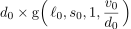
![[d_0] = \mathit{mass} / \mathit{length}^3](https://alexchinco.com/wp-content/ql-cache/quicklatex.com-fb609277c35420eda67b1f68b2be838c_l3.svg "Rendered by QuickLaTeX.com") times
times ![[\mathrm{g}( \, \ell_0, \, s_0, \, 1, \, v_0/d_0 \, )] = \mathit{length}^4 / \mathit{time}^2](https://alexchinco.com/wp-content/ql-cache/quicklatex.com-6e4fa27f927c5fe091c6ad3c6c41280d_l3.svg "Rendered by QuickLaTeX.com") . This yields a combined dimension of
. This yields a combined dimension of  for the right-hand side, which is exactly what we’re after.
 ,
,  , and
, and  , then we would need to multiply the right-hand side by an additional factor of
  to preserve dimensional consistency:
 and
and  are chosen to balance the dimensions on either side of the equal sign in Equation (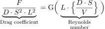
![[F/ (D \cdot S^2 \cdot L^2)] = 1](https://alexchinco.com/wp-content/ql-cache/quicklatex.com-e24794a11b50daba79deb4e93a8fc5a1_l3.svg "Rendered by QuickLaTeX.com") , and commonly called the “drag coefficient”. The input to
, and commonly called the “drag coefficient”. The input to  is called the
  , and is also dimensionless,
 ![[L \cdot \{(D \cdot S) / V\}] = 1](https://alexchinco.com/wp-content/ql-cache/quicklatex.com-657bbb8b62d33d460a4edbdcee13307d_l3.svg "Rendered by QuickLaTeX.com") .
. was a function of four variables.
  is a function of a single variable. These textbooks argue that it’s easier to estimate
  , combines the four other inputs
 -times as viscous as sea water, like honey
  , do you observe a similar drag coefficient on your 1ft model submarine?
 , that might predict the cross-section of returns. And you’ve regressed returns on
  of your choosing (i.e., using data on some specific
 .
.  . Assets with higher
  . Let
. Let  denote the collection of all out-of-sample market environments that your colleagues might examine.
 . But, even if
  where
where  , then one of your colleagues will surely discover it and you’ll look utterly foolish when he tells the world. You only want to publish if
![\lambda \in (0, \, 1]](https://alexchinco.com/wp-content/ql-cache/quicklatex.com-8809687cecc74fe1171a83cf272a2b6e_l3.svg "Rendered by QuickLaTeX.com") captures the
captures the  , the
, the 
 , are the same in every market environment.
  is an
is an  captures its affect on returns.
 , or
, or  , but not both in investors’ model. If
  is the same in every environment—i.e., in every time period, country, etc. If
 ![\begin{equation*} \mathsf{\Theta} = \{ \, (\theta, \, \vartheta) \in [-1, \, 1]^2 \, | \, 1_{\{\theta \neq 0\}} + 1_{\{ \vartheta \neq 0 \}} = 1 \, \} \end{equation*}](https://alexchinco.com/wp-content/ql-cache/quicklatex.com-147826db88789fbaa34cbd4cfe7fadd3_l3.svg "Rendered by QuickLaTeX.com")
 might take on.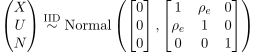
![\Corr_e[X, \, N] = \Corr_e[U, \, N] = 0](https://alexchinco.com/wp-content/ql-cache/quicklatex.com-47c90352512a0652b8564fe14b7a165f_l3.svg "Rendered by QuickLaTeX.com") . However,
. However, ![\Corr_e[X, \, U] = \rho_e \neq 0](https://alexchinco.com/wp-content/ql-cache/quicklatex.com-c45e4d84f15e3f3d01562364a37efa7f_l3.svg "Rendered by QuickLaTeX.com") . Moreover, this correlation can differ across market environments. In other words,
. Moreover, this correlation can differ across market environments. In other words, ![\Exp_e[R] = 0](https://alexchinco.com/wp-content/ql-cache/quicklatex.com-154d15b5f5213e5d5efcfdadd31e9904_l3.svg "Rendered by QuickLaTeX.com") , in every market environment. I’m making this assumption to keep the math simple. If it really bothers you, just think about
, in every market environment. I’m making this assumption to keep the math simple. If it really bothers you, just think about  as an asset’s residual return that unexplained by other trading signals. Let’s also assume that
 ![\Var_e[R] = 1](https://alexchinco.com/wp-content/ql-cache/quicklatex.com-05f48a467f09cd3c96ea79ff23d8e7bd_l3.svg "Rendered by QuickLaTeX.com") in every market environment for the same reasons. This assumption implies that
in every market environment for the same reasons. This assumption implies that  .
.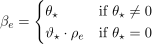
 in every environment. Or it might be that you estimated
  . These are the two possible explanations.
 merely because
 ![\mathbb{S}\mathrm{ign}[\rho_e] = \mathbb{S}\mathrm{ign}[\rho_{e'}]](https://alexchinco.com/wp-content/ql-cache/quicklatex.com-20f707e8a001c807a340851f86a3caf4_l3.svg "Rendered by QuickLaTeX.com") . Under this explanation, it’s possible to imagine market environments where
. Under this explanation, it’s possible to imagine market environments where ![\mathbb{S}\mathrm{ign}[\rho_e] \neq \mathbb{S}\mathrm{ign}[\rho_{e'}]](https://alexchinco.com/wp-content/ql-cache/quicklatex.com-4a72a58208d2dadf7a8b2e80dbb94383_l3.svg "Rendered by QuickLaTeX.com") .
.![\Corr_e[X, \, U] = \rho_e](https://alexchinco.com/wp-content/ql-cache/quicklatex.com-966e15116fb9b45448c8c1b3bfcbfebd_l3.svg "Rendered by QuickLaTeX.com") might take on:
might take on:![\begin{equation*} \mathsf{P}_e = \{ \, \rho \in [-1, \, 1] \, | \, \text{it could be that $\Corr_e[X, \, U] = \rho$ in market environment $e$} \, \} \end{equation*}](https://alexchinco.com/wp-content/ql-cache/quicklatex.com-4a8895983e5b3ab6b9413030327620c0_l3.svg "Rendered by QuickLaTeX.com")
 , consists of a set of structural parameters,
  ; a range of possible values for the correlation between
  ; and, a particular choice for this value,
  .
. have the same structural parameters,
  , then the cross-sectional slope coefficient will be the same in both environments,
  . Yet, you will interpret the slope coefficient differently in each environment if
  . By analogy, medical researchers will draw different conclusions about a drug’s efficacy from an
  , then
  in such an environment. By contrast, if
  , then
  could be explained either by
  .
. consists of an arbitrarily small neighborhood around zero. The omitted variable
  of the variation in returns across assets. That would occur if
  since we are assuming
 ![\Var_{e'}[R] = 1](https://alexchinco.com/wp-content/ql-cache/quicklatex.com-326c2fd196c04d049539e17773d8adf7_l3.svg "Rendered by QuickLaTeX.com") . Hence, if
. Hence, if  and
and  due to a spurious correlation, then this correlation must be bounded away from zero:

 . If
. If  and we say that market environment
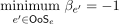
 ![\begin{equation*} \mathsf{OoS}_e = \{ \, e' = (\theta, \, \vartheta; \mathsf{P}, \, \rho ) \, | \, \theta, \, \vartheta \in \mathsf{\Theta}_e \text{ and } \rho \in [-1, \, 1] = \mathsf{P} \, \} \end{equation*}](https://alexchinco.com/wp-content/ql-cache/quicklatex.com-1d6b20fe0eea59546eb02f1b15fb904e_l3.svg "Rendered by QuickLaTeX.com")
![\rho \in [-1, \, 1]](https://alexchinco.com/wp-content/ql-cache/quicklatex.com-77c25ee638e8e1c0937341be55681124_l3.svg "Rendered by QuickLaTeX.com") .
. in every out-of-sample market environment. The left-hand side of Equation (
 or it could be that
  . If the latter is true, then we would say that
  reflects a spurious correlation. And to make this spurious correlation look as bad as possible out-of-sample, other researchers should look for a market environment
  :
:
 in lots of different market environments
  in many different market environments
  . For example, if
  in more than half of all possible out-of-sample environments, then there’s no way for
  since we know that
  in every remaining market environment as we saw in Equation (
 in one of the remaining environments in
  , then simply doing lots of in-sample checks isn’t a viable research strategy on its own. It certainly doesn’t hurt. But it DOES NOT tell you anything about out-of-sample robustness in the setup thusfar.
 . Such identifying assumptions can be hard to stomach. However, the assumption that you would need to make for in-sample robustness to guarantee out-of-sample robustness is even less palatable.
  in some specific market environment, you would need to assume that
 ![\beta = \frac{\Cov[R_{t+1}, \, \Delta \log C_{t+1}]}{\Var[\Delta \log C_{t+1}]}](https://alexchinco.com/wp-content/ql-cache/quicklatex.com-cf8f88949b04673c5f3c3bf0a2196394_l3.svg "Rendered by QuickLaTeX.com") :
:![\begin{equation*} \Exp[R_{t+1}] = R_f + \lambda \cdot \beta \end{equation*}](https://alexchinco.com/wp-content/ql-cache/quicklatex.com-07781edb80d028bbaa211146aa957141_l3.svg "Rendered by QuickLaTeX.com")
![\begin{equation*} \begin{split} \text{maximize} &\quad \Exp_0\left[ \, {\textstyle \sum_{t=0}^{\infty}} \, e^{-\rho \cdot t} \cdot \mathrm{U}(C_t) \, \right] \\ \text{subject to} &\quad \parbox[b]{1.00cm}{\raggedleft $\mathrm{U}(C)$} = {\textstyle \frac{C^{1-\gamma} - 1}{1-\gamma}} \\ &\quad \parbox[b]{1.00cm}{\raggedleft $W_t$} \geq C_t + P_t \cdot S_t + B_t \\ &\quad \parbox[b]{1.00cm}{\raggedleft $W_{t+1}$} = (P_{t+1} + D_{t+1}) \cdot S_t + (1+R_f) \cdot B_t \\ &\quad \parbox[b]{1.00cm}{\raggedleft $D_{t+1}$} = D_t \cdot e^{\mu + \sigma \cdot \varepsilon_{t+1}} \quad \varepsilon_{t+1} \overset{\scriptscriptstyle \textnormal{IID}}{\sim} \mathrm{Normal}(0, \, 1) \\ \text{on inputs} &\quad \parbox[b]{1.00cm}{\raggedleft $W_0$}, \, D_0 \! > \! 0, \, \mu \! > \! \rho \! > \! 0, \, \sigma \! > \! 0, \, \gamma \! > \! 1, \, R_f \! > \! 0 \end{split} \end{equation*}](https://alexchinco.com/wp-content/ql-cache/quicklatex.com-c2fca7c8b121142973e07af550a22f34_l3.svg "Rendered by QuickLaTeX.com")
 . (Line 2; Preferences) The investor has power utility with risk aversion parameter,
  . (Line 3; Budget Constraint) At time
  , the investor must have enough wealth
  to cover his consumption
  AND to pay for the
  shares of the market that he buys at a price of
  dollars per share AND to pay for the
  dollars he invests in riskless bonds. (Line 4; Wealth Evolution) The investor’s will receive a
  dollar dividend for each share of the market he bought at time
  dollars AND he will earn the riskfree rate of
  on each dollar he invested in bonds at time
  per period, and it has a per period volatility of
  .
.![\begin{equation*} P_t = \Exp \left[ \, e^{-(\rho + \gamma \cdot \Delta \log C_{t+1})} \times (D_{t+1} + P_{t+1}) \, \right] \end{equation*}](https://alexchinco.com/wp-content/ql-cache/quicklatex.com-3c094c8a372d06752f002db4ef14191b_l3.svg "Rendered by QuickLaTeX.com")
 (total payout = the dividend
  , and his aversion to fluctuations in consumption,
  .
. . And, if we define the return to holding a share of the market portfolio as
  , then
 ![\Exp[R_{t+1}]](https://alexchinco.com/wp-content/ql-cache/quicklatex.com-f5da68dc4eb18b2d54576ec35f857ef9_l3.svg "Rendered by QuickLaTeX.com") , should be equal to the riskfree rate plus a term proportional to the market’s consumption beta,
, should be equal to the riskfree rate plus a term proportional to the market’s consumption beta, ![\hat{\Exp}[R_{t+1}]](https://alexchinco.com/wp-content/ql-cache/quicklatex.com-5a2e7f70835c4d14a126363ee4e2c643_l3.svg "Rendered by QuickLaTeX.com") and
and  using historical data on market returns and aggregate consumption.

You must be logged in to post a comment.