Notes: Ang, Hodrick, Xing, and Zhang (2006)

1. Introduction

In this post I work through the main results in Ang, Hodrick, Xing, and Zhang (2006) which shows not only that i) stocks with more exposure to changes in aggregate volatility have higher average excess returns, but also that ii) stocks with more idiosyncractic volatility relative to the Fama and French (1993) $3$ factor model have lower excess returns. The first result is consistent with existing asset pricing theories; whereas, the second result is at odds with almost any mainstream asset pricing theory you might write down. Idiosyncratic risk should not be priced. This paper together with Campbell, Lettau, Malkiel, and Xu (2001) (see my earlier post) set off an investigation into the role of idiosyncratic risk in determining asset prices. One possibility is that idiosyncratic risk is just a proxy for exposure to aggregate risk. i.e., perhaps it’s the firms with the highest exposure to aggregate return volatility that also have the highest idiosyncratic volatility. Interestingly, Ang, Hodrick, Xing, and Zhang (2006) show that this is not the case via a double sort on both aggregate and idiosyncratic volatility exposure giving evidence that these are $2$ separate risk factors. The code I use to replicate the results in Ang, Hodrick, Xing, and Zhang (2006) and create the figures can be found here.

2. Theoretical Motivation

The discount factor view of asset pricing says that:

(1) $\begin{align*} 0 = \mathrm{E}[m \cdot r_n] \quad \text{for all } n=1,2,\ldots,N \end{align*}$

where $\mathrm{E}(\cdot)$ denotes the expectation operator, $m$ denotes the stochastic discount factor, and $r_n$ denotes asset $n$ ‘s excess return. Equation (1) reads: “In the absence of margin requirements and transactions costs, it costs you $\mathdollar 0$ today to borrow at the riskless rate, buy a stock, and hold the position for $1$ period.” Asset pricing theories explain why average excess returns, $\mathrm{E}[r_n]$ , vary across assets even though they all have the same price today by construction (see my earlier post).

Suppose each asset’s excess returns are a function of a risk factor $x$ , $\mathrm{R}_n(x)$ , and noise, $z_n \overset{\scriptscriptstyle \mathrm{iid}}{\sim} \mathrm{N}(0,\sigma_z^2)$ :

(2) $\begin{align*} r_n &= \mathrm{R}_n(x) + z_n \\ &= \mathrm{R}_n(\mu_x) + \mathrm{R}_n'(\mu_x) \cdot (x - \mu_x) + \frac{1}{2} \cdot \mathrm{R}_n''(\mu_x) \cdot (x - \mu_x)^2 + \text{``h.o.t.''} + z_n \\ &\approx \alpha_n + \beta_n \cdot (x - \mu_x) + \frac{\gamma_n}{2} \cdot (x - \mu_x)^2 + z_n \end{align*}$

where I assume for simplicity that the only risk factor is the value-weighted excess return on the market so that $\mu_x \approx 6{\scriptstyle \%/\mathrm{yr}}$ and $\sigma_x \approx 16{\scriptstyle \%/\mathrm{yr}}$ . I use a Taylor expansion to linearize the function $\mathrm{R}_n(x)$ around the point $x = \mu_x$ and assume $\mathrm{O}(x - \mu_x)^3$ terms are negligible so $\mathrm{E}[r_n] = \alpha_n + \sfrac{\gamma_n}{2} \cdot \sigma_x^2$ and $\mathrm{Var}[r_n] = \beta_n^2 \cdot \sigma_x^2 + \sigma_z^2$ . This means that if the excess return on the market is $\sfrac{16{\scriptstyle \%}}{\sqrt{252}} \approx 1{\scriptstyle \%/\mathrm{day}}$ larger than expected, then asset $n$ ‘s expected excess returns will be $\beta_n{\scriptstyle \%}$ larger.

Any asset pricing theory says that each asset’s expected excess return should be proportional to how much the asset comoves with the risk factor, $x$ :

(3) $\begin{align*} \mathrm{E}[r_n] = \alpha_n + \frac{\gamma_n}{2} \cdot \sigma_x^2 = \underbrace{\text{Constant} \times \beta_n}_{\text{Predicted}} \end{align*}$

where the constant of proportionality, $\text{Constant} = c \cdot (\sfrac{\mathrm{Var}[m]}{\mathrm{E}[m]})$ , depends on the exact asset pricing model. Equation (3) says that if you ran a regression of each stock’s excess returns on the aggregate risk factor:

(4) $\begin{align*} r_{n,t} = \widehat{\alpha}_n + \widehat{\beta}_n \cdot x_t + \mathit{Error}_{n,t} \end{align*}$

then the estimated intercept for each stock should be:

(5) $\begin{align*} \widehat{\alpha}_n = \frac{\gamma_n}{2} \cdot \sigma_x^2 - \beta_n \cdot \mu_x \end{align*}$

Thus, each stock’s average excess returns may well be related to its exposure to aggregate volatility since $\sigma_x$ shows up in the expression for $\widehat{\alpha}_n$ ; however, idiosyncratic volatility, $\sigma_z$ , better not be priced since it shows up nowhere above.

3. Aggregate Volatility

Ang, Hodrick, Xing, and Zhang (2006) show that stocks with more exposure to aggregate volatility have lower average excess returns. i.e., that the coefficient $\gamma_n < 0$ . The authors actually look at each stock’s exposure to changes in aggregate volatility. To see how this changes the math, consider rewriting the intercept above as:

(6) $\begin{align*} \widehat{\alpha}_n = \mathrm{A}_n(\Delta \sigma_x) &= \alpha_n + \frac{\gamma_n}{2} \cdot \left(\langle \sigma_x \rangle + \Delta \sigma_x \right)^2 \end{align*}$

Using this formulation, we can look at how perturbing $\mathrm{A}_n(\Delta \sigma_x)$ around its mean with some small $\Delta \sigma_x$ will impact the estimated intercept:

(7) $\begin{align*} \mathrm{A}_n(\Delta \sigma_x) &= \mathrm{A}_n(0) + \mathrm{A}_n'(0) \cdot \Delta \sigma_x + \cdots \\ &\approx \left[ \alpha_n + \frac{\gamma_n}{2} \cdot \langle\sigma_x\rangle^2 \right] + \gamma_n \cdot \langle\sigma_x\rangle \cdot \Delta \sigma_x \end{align*}$

Since $\langle \sigma_x \rangle > 0$ by definition, $(\sfrac{\gamma_n}{2}) \cdot \langle \sigma_x \rangle^2$ and $\gamma_n \cdot \langle \sigma_x \rangle$ will have the same sign. Thus, testing for whether exposure to changes in aggregate volatility is priced is tantamount to testing for whether exposure to aggregate volatility is priced.

The authors proceed in $5$ steps. First, they calculate the changes in aggregate volatility time series using changes in the daily options implied volatility:

(8) $\begin{align*} \Delta \sigma_{x,d+1} = \mathit{VXO}_{d+1} - \mathit{VXO}_d \qquad \text{with} \qquad \mathrm{E}[\Delta \sigma_{x,d+1}] = 0.01{\scriptstyle \%}, \, \mathrm{StD}[\Delta \sigma_{x,d+1}] = 2.65{\scriptstyle \%} \end{align*}$

If the VXO is $4.33{\scriptstyle \%}$ , then options markets expect the S&P 100 to move up or down $4.33{\scriptstyle \%}$ over the next $30$ calendar days. The authors use the VXO contract price rather than the VIX contract price because it has a longer time series dating back to 1986. The only difference between the $2$ contracts is that the VXO quotes the options implied volatility on the S&P 100; whereas, the VIX quotes the options implied volatility on the S&P 500. Daily changes in the $2$ contract prices have a correlation of $0.81$ over the sample period from January 1986 to December 2012 as shown in the figure below.

Second, the authors compute each stock’s exposure to changes in aggregate volatility by running a regression for each stock $n \in \{1,2,\ldots,N\}$ using the daily data in month $(m-1)$ :

(9) $\begin{align*} r_{n,d} = \widehat{\alpha}_n + \widehat{\beta}_{n} \cdot x_d + \widehat{\gamma}_{n} \cdot \Delta \sigma_{x,d} + \mathit{Error}_{n,d} \end{align*}$

Estimated coefficients are related to underlying deep parameters by:

(10) $\begin{align*} \widehat{\alpha}_n &= \frac{\gamma_n}{2} \cdot \langle \sigma_x \rangle^2 - \beta_n \cdot \mu_x \\ \widehat{\beta}_n &= \beta_n \\ \widehat{\gamma}_n &= \gamma_n \cdot \langle \sigma_x \rangle \end{align*}$

The daily market excess return, $x_d$ , is the excess return on the CRSP value-weighted market index. I include AMEX, NYSE, and NASDAQ stocks with $\geq 17$ daily observations in month $(m-1)$ in my universe of $N$ stocks.

Third, the authors sort the $N$ stocks satisfying the data constraints in month $(m-1)$ into $5$ value-weighted portfolios based on their estimated $\widehat{\gamma}_{n}$ . Note that because the factor $\langle \sigma_x \rangle$ is common to all stocks in month $(m-1)$ , this sort effectively organizes stocks by their true exposure to aggregate volatility, $\gamma_n$ . For each portfolio $j \in \{\text{L},2,3,4,\text{H}\}$ with $j = \text{L}$ denoting the stocks with the lowest aggregate volatility exposure and $j = \text{H}$ denoting the stocks with the highest aggregate volatility exposure, the authors then calculate the daily portfolio returns in month $m$ . The figure above shows the cumulative returns to each of these $5$ portfolios. It reads that if you invested $\mathdollar 1$ in the low aggregate volatility exposure portfolio in January 1986, then you would have over $\mathdollar 200$ more dollars in December 2012 than if you had invested that same $\mathdollar 1$ in the high aggregate volatility exposure portfolio. What’s more, each portfolio’s exposure to the excess return on the market is not explaining its performance. The figure below reports the estimated intercepts for each $j \in \{\text{L},2,3,4,\text{H}\}$ from the regression:

(11) $\begin{align*} r_{j,m} = \widehat{\alpha}_j + \widehat{\beta}_j \cdot x_m + \mathit{Error}_{j,m} \end{align*}$

and indicates that abnormal returns are decreasing in the portfolio’s exposure to aggregate volatility.

Fourth, in order to test whether the spread in portfolio abnormal returns is actually explained by contemporaneous exposure to aggregate volatility, the authors then create an aggregate volatility factor mimicking portfolio. They estimate the regression below using the daily excess returns on each of the $5$ aggregate volatility exposure portfolios in each month $m$ :

(12) $\begin{align*} \Delta \sigma_{x,d} = \widehat{\kappa} + \sum_{j=\text{L}}^{\text{H}} \widehat{\lambda}_{j} \cdot r_{j,d} + \mathit{Error}_d \end{align*}$

and store the parameter estimates for $\begin{bmatrix} \widehat{\lambda}_1 & \widehat{\lambda}_2 & \widehat{\lambda}_3 & \widehat{\lambda}_4 & \widehat{\lambda}_5 \end{bmatrix}^{\top}$ . They then define the factor mimicking portfolio return at daily horizon in month $m$ as:

(13) $\begin{align*} f_d = \sum_{j=\text{L}}^{\text{H}} \widehat{\lambda}_{j} \cdot r_{j,d} \end{align*}$

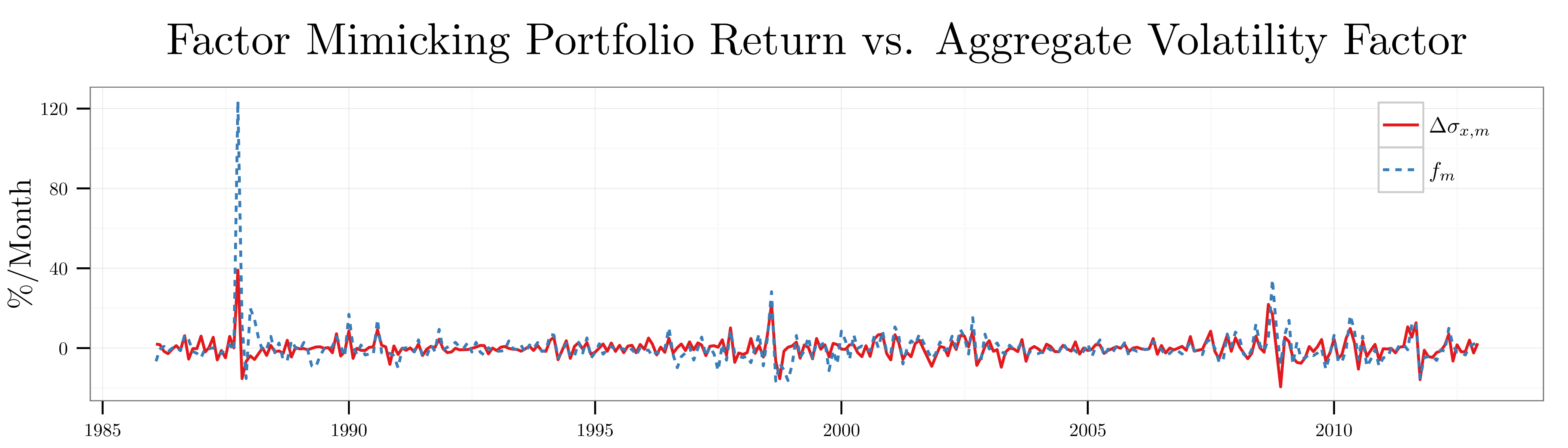
The figure below plots the factor mimicking portfolio returns against the underlying changes in aggregate volatility at the monthly level. The $2$ data series line up relatively closely; however, the factor mimicking portfolio is much too volatile during crises such as Black Monday in 1987.

Fifth and finally, the authors check whether or not each of the $5$ aggregate volatility portfolio’s returns are positively correlated with contemporaneous movements in the aggregate volatility factor mimicking portfolio at the monthly horizon. To do this, they cumulate up daily excess returns on the factor mimicking portfolio and the aggregate volatility exposure sorted portfolios to get monthly returns:

(14) $\begin{align*} f_m &= \sum_{d=1}^{22} f_d \\ r_{j,m} &= \sum_{d=1}^{22} r_{j,d} \quad \text{for all } j \in \{\text{L},2,3,4,\text{H}\} \end{align*}$

Then, they run the regression below at a monthly horizon over full sample:

(15) $\begin{align*} r_{j,m} = \widehat{\zeta}_j + \widehat{\eta}_j \cdot x_m + \widehat{\theta}_j \cdot f_m + \mathit{Error}_{j,m} \end{align*}$

I report the estimated $\widehat{\theta}_j$ coefficients in the figure below. Consistent with the idea that exposure to aggregate volatility is driving the disparate excess returns of the $5$ test portfolios, I find that each portfolio loads positively on monthly movements in the factor mimicking portfolio.

4. Idiosyncratic Volatility

Ang, Hodrick, Xing, and Zhang (2006) also show that stocks with more idiosyncratic volatility have lower average excess returns. This should not be true under the standard theory outlined in Section 2 above. To measure idiosyncratic volatility, the authors run the regression below at the daily level in month $(m-1)$ for each stock $n = 1,2,\ldots,N$ :

(16) $\begin{align*} r_{n,d} = \widehat{\alpha}_n + \widehat{\boldsymbol \beta}_n^{\top} \cdot \mathbf{x}_d + \mathit{Error}_{n,d} \end{align*}$

where the risk factors are the excess return on the value weighted market portfolio, the excess return on a size portfolio, and the excess return on a value portfolio as dictated by Fama and French (1993):

(17) $\begin{align*} \mathbf{x}_d^{\top} = \begin{bmatrix} r_{\mathrm{Mkt},d} & r_{\mathrm{SmB},d} & r_{\mathrm{HmL},d} \end{bmatrix} \end{align*}$

For each stock listed on the AMEX, NYSE, or NASDAQ stock exchange with $\geq 17$ daily observations in month $(m-1)$ , the authors then calculate the measure of idiosyncratic volatility below:

(18) $\begin{align*} \sigma_{z,n} &= \mathrm{StD}[\mathit{Error}_{n,d}] \end{align*}$

The authors sort the $N$ stocks satisfying the data constraints in month $(m-1)$ into $5$ value-weighted portfolios based on their estimated $\sigma_{z,n}$ values. The figure above reports the cumulative returns to these $5$ test portfolios. The figure reads that if you invested $\mathdollar 1$ in the low idiosyncratic volatility portfolio in January 1963, then you would have over $\mathdollar 100$ more in December 2012 than if you had invested in the high idiosyncratic volatility portfolio. The figure below reports the estimated abnormal returns, $\widehat{\alpha}_j$ , for each of the idiosyncratic volatility portfolios over the full sample and confirms that the poor performance of the high idiosyncratic volatility portfolio cannot be explained by exposure to common risk factors.

5. Are They Related?

I conclude by discussing the obvious follow-up question: “Are these $2$ phenomena related?” After all, it could be the case that the firms with the highest exposure to aggregate return volatility also have the highest idiosyncratic volatility and vice versa. Ang, Hodrick, Xing, and Zhang (2006) show that this is not the case via a double sort. i.e., they show that within each aggregate volatility exposure portfolio, the stocks with the lowest idiosyncratic volatility outperform the stocks with the highest idiosyncratic volatility. Similarly, they show that within each idiosyncratic volatility portfolio, the stocks with the lowest aggregate volatility exposure outperform the stocks with the highest aggregate volatility exposure. Thus, the motivation driving investors to pay a premium for stocks with high aggregate volatility exposure is different from the motivation driving investors to pay a premium for stocks with high idiosyncratic volatility.

Indeed, you can pretty much guess this fact from the cumulative return plots in Sections $3$ and $4$ where the red lines denoting the low exposure portfolios behave in completely different ways. e.g., the low aggregate volatility exposure portfolio returns behave more or less like the high aggregate volatility exposure portfolio returns but with a higher mean. By contrast, the low idiosyncratic volatility portfolio returns are a much different time series with dramatically less volatility. Interestingly, if the authors sort on total volatility in month $(m-1)$ rather than idiosyncratic volatility, then results are identical; however, the results to not carry through if you sort on $R^2$ in month $(m-1)$ . e.g., suppose you ran the same regression at the daily level in month $(m-1)$ for each stock $n = 1,2,\ldots,N$ :

(19) $\begin{align*} r_{n,d} = \widehat{\alpha}_n + \widehat{\boldsymbol \beta}_n^{\top} \cdot \mathbf{x}_d + \mathit{Error}_{n,d} \end{align*}$

(20) $\begin{align*} \mathbf{x}_d^{\top} = \begin{bmatrix} r_{\mathrm{Mkt},d} & r_{\mathrm{SmB},d} & r_{\mathrm{HmL},d} \end{bmatrix} \end{align*}$

Then, for each stock you computed the $R^2$ statistic measuring the fraction of the total variation in each stock’s excess returns that is explained by movements in the risk factors:

(21) $\begin{align*} R^2 &= 1 - \frac{\sum_{d=1}^{22}(r_{n,d} - \{\widehat{\alpha}_n + \widehat{\boldsymbol \beta}_n^{\top} \mathbf{x}_d\})^2}{\sum_{d=1}^{22}(r_{n,d} - \langle r_{n,d} \rangle)^2} \end{align*}$

If you group stocks into $5$ portfolios based on their $R^2$ over the previous month, the figure above shows that there is no monotonic spread in the abnormal returns. Thus, the idiosyncratic volatility results seem to be more about volatility and less about the explanatory power of the Fama and French (1993) factors.