A frictionless mean-variance model predicts an aggregate demand elasticity of  . Suppose the level of the stock market rises by
  on no fundamental news. It’s now more expensive to buy stocks, but nothing’s changed to make the anticipated payout next year more desirable. Textbook theory says that investors ought to look at this drop in forecasted returns and dump
  of their holdings. The data disagrees. There, the aggregate demand elasticity is much much lower. Gabaix-Koijen estimate
  .
.
To get an elasticity that low, investors need to look at the increase in today’s price and shrug their shoulders. In this note, I show that this is exactly what happens when investors rely on trailing PE ratios when setting price targets. I show that this one simple observation is able to generate a predicted demand elasticity of  . This is well within spitting distance of the estimated
  .
.
The trailing-PE mechanism is kind of like a dogmatic-learning story. Think about a Bayesian investor who treats the current price level as a very precise signal about next year’s payout. Such an investor would face the same demand curve as a trailing-PE user. But the analogy isn’t perfect. The trailing-PE approach doesn’t force next year’s price target to agree with next year’s dividend forecast in present-value terms. When the current price rises, the target rises with it, but the dividend forecast doesn’t budge.
Demand Elasticity
Suppose an asset’s current price changes a tiny bit for non-fundamental reasons. Suppose an investor’s forecasting and allocation rules remain unchanged. How much will her desired position change in response? The answer to this question is called the demand elasticity
(1) 
A change in the current price of an asset affects the investor’s demand in two ways. There’s a rebalancing channel,  , which creates a difference between stock-level and aggregate demand elasticities. There’s also a belief channel. A change in today’s price can impact the investor’s views about next year’s payoff. This is the
  term, and it pins down the overall level. Here’s where this formula comes from.
Let  denote an asset’s share of an investor’s wealth. Hold her forecasted return fixed, which switches off the belief channel and keeps a fixed fraction of her wealth in the asset. Under this assumption, a price rise means the same number of shares now ties up more of her wealth. Restoring her target weight means trimming shares and parking the proceeds in the rest of the portfolio.
If the investor already holds the asset, then the trim is partly cancelled. The increase in the current price will also revalue her existing position, raising her wealth by  percent
(2) 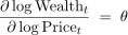
This change lifts her target dollar allocation for the asset by the same percent.
The net sale is percent of her shares, which is exactly the share of her portfolio held in other assets. That is the room she has to rebalance into. For a single stock inside a diversified portfolio, we have  and
and  . For an investor choosing how much to invest in the market as a whole, we have
  and
and  . The whole term vanishes.
The belief channel starts with a mapping from the current price to beliefs about future returns. I write the investor’s forecasts as ![\mathbb{F}_t[\cdot]](https://alexchinco.com/wp-content/ql-cache/quicklatex.com-c41565336510190935c557bf9fb935a6_l3.svg "Rendered by QuickLaTeX.com") , rather than
, rather than ![\mathbb{E}_t[\cdot]](https://alexchinco.com/wp-content/ql-cache/quicklatex.com-1bc50689ea90ae6d13bcd8df908f8841_l3.svg "Rendered by QuickLaTeX.com") , because forecasts don’t need to come from a well-posed probability space. A forecast is just a number that the investor writes down.
, because forecasts don’t need to come from a well-posed probability space. A forecast is just a number that the investor writes down.
A share bought today for  delivers the dollar payout
  next year. The realized gross return on this investment will be
(3) 
If you expand the exponential expression around the steady state, then you get the following first-order approximation for the net return
(4) 
I use the Gabaix-Koijen calibration values: a long-run dividend yield  and an average forecasted return
  . A rise in the payout raises the gross return by
  , and a rise in the current price lowers the return by the same amount.
Assumption A1. The investor forecasts the asset’s future payout with a rule ![\mathbb{F}_t[\mathrm{Payout}_{t+1}]](https://alexchinco.com/wp-content/ql-cache/quicklatex.com-111a0d12dfec50d41e34bbbaa79df4c8_l3.svg "Rendered by QuickLaTeX.com") that is differentiable in
that is differentiable in  , and her return forecast is given by
(5) ![\begin{equation*}\mathbb{F}_t[\mathrm{Ret}_{t+1}] \;=\; (1 {+} \overline{\mathrm{DY}}) \cdot \big( \log \mathbb{F}_t[\mathrm{Payout}_{t+1}] \,-\, \log \mathrm{Price}_t \big) \,+\, \mathrm{constant}\end{equation*}](https://alexchinco.com/wp-content/ql-cache/quicklatex.com-68cf1d9df05c606dfe75a5dad70d90e8_l3.svg "Rendered by QuickLaTeX.com")
Notice what A1 does not assume: present-value logic. Nothing forces today’s price to equal her payout forecast discounted at a required return, so her payout forecast can move independently of the multiple, and a shock to ![\mathbb{F}_t[\mathrm{EPS}_{t+1}]](https://alexchinco.com/wp-content/ql-cache/quicklatex.com-c440ee3ecfec6def0744b4f2e57d6f34_l3.svg "Rendered by QuickLaTeX.com") need not have any impact on the PE. A1 does not impose Gordon logic, either directly or approximately as in Campbell-Shiller. A1 pins down the investor’s return forecast for next year as a function of her payout forecast and the current price.
need not have any impact on the PE. A1 does not impose Gordon logic, either directly or approximately as in Campbell-Shiller. A1 pins down the investor’s return forecast for next year as a function of her payout forecast and the current price.
Differentiating gives the belief drag,  . This parameter represents the price sensitivity of the investor’s forecasted return for the upcoming year
(6) ![\begin{equation*}\mu \;=\; {-}\frac{\partial \, \mathbb{F}_t[\mathrm{Ret}_{t+1}]}{\partial \log \mathrm{Price}_t} \;=\; (1 {+} \overline{\mathrm{DY}}) \times \bigg( 1 \,-\, \frac{\partial \log \mathbb{F}_t[\mathrm{Payout}_{t+1}]}{\partial \log \mathrm{Price}_t} \bigg)\end{equation*}](https://alexchinco.com/wp-content/ql-cache/quicklatex.com-23c4dc8ca23e0cb2d33b37c60d21ef47_l3.svg "Rendered by QuickLaTeX.com")
If the current price goes up by and nothing else changes, how much will the investor’s return forecast fall in response?
In a frictionless mean-variance model, the investor observes the asset’s current price. But this information doesn’t impact how she values the stock. Her payout forecast is built from fundamentals alone, so ![\frac{\partial \log \mathbb{F}_t[\mathrm{Payout}_{t+1}]}{\partial \log \mathrm{Price}_t} = 0](https://alexchinco.com/wp-content/ql-cache/quicklatex.com-eaed5236194bda61fd36d93e67ce572e_l3.svg "Rendered by QuickLaTeX.com") and
and  . She suffers the full drag.
The belief drag has units of percent per year. is a change in the asset’s anticipated return over the next twelve months. The average forecasted return  has the same units. So the ratio
  is dimensionless, which an elasticity term has to be. The two terms combine to form the elasticity of the forecasted return with respect to the current price.
A textbook investor in a frictionless mean-variance model has belief drag  . A increase in the current price level will lower her forecasted return for next year by
  . When we compare this effect to the long-run average return forecast,
  , we get a relative change of
  . The original drag on the asset’s forecasted return may not sound like much, but it’s a big deal compared to the average return forecast.
measures the percent decline in the forecasted return when the price rises . The parameter  converts this elasticity of forecasted returns into an elasticity of demand. You might think this conversion requires a full-fledged asset-pricing model. It turns out any allocation rule with the following form will do.
Assumption A2. The dollar allocation is ![\mathrm{Wealth}_t \times w\big(\mathbb{F}_t[\mathrm{Ret}_{t+1}]\big)](https://alexchinco.com/wp-content/ql-cache/quicklatex.com-3983a52d81dd9f09a97a42e02287810a_l3.svg "Rendered by QuickLaTeX.com") for a smooth increasing rule
for a smooth increasing rule  .
.
The number of shares that the investor demands can be written as  times the ratio of her initial wealth and the asset’s share price
(7) ![\begin{equation*}\mathrm{Dmnd}_t \;=\; w\big(\mathbb{F}_t[\mathrm{Ret}_{t+1}]\big) \times \bigg\{ \frac{\mathrm{Wealth}_t}{\mathrm{Price}_t}\bigg\}\end{equation*}](https://alexchinco.com/wp-content/ql-cache/quicklatex.com-4f57c4dc0b5faeeddc7336ef4d130d58_l3.svg "Rendered by QuickLaTeX.com")
e.g., mean-variance preferences deliver the special case  .
.
 represents the elasticity of the investor’s dollar position in the asset with respect to her forecasted return next year evaluated at the asset’s long-run average forecast
(8) 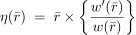
e.g., if an asset’s forecasted return improves by , from to  , the investor scales her dollar allocation in the asset up by
  .
.
Note that  to leading order. For mean-variance preferences, we have
  exactly. To see why, take any smooth rule with
  . A Taylor expansion gives
  , so
, so
(9) 
If , then  and
and  for all
  . Hence, we have for all . However, any preference specification with
  and
and  would do the same to leading order.
The pieces now assemble by the chain rule. First, take logs of the demand rule
(10) ![\begin{equation*}\log \mathrm{Dmnd}_t \;=\; \log w\big(\mathbb{F}_t[\mathrm{Ret}_{t+1}]\big) \,+\, \log \mathrm{Wealth}_t \,-\, \log \mathrm{Price}_t\end{equation*}](https://alexchinco.com/wp-content/ql-cache/quicklatex.com-87e8d4f51c5d13fbd8a0020d84bd4177_l3.svg "Rendered by QuickLaTeX.com")
Next, differentiate each term with respect to . The wealth term contributes and the price term contributes  . Together they are the rebalancing channel, .
The first ![\log w\big(\mathbb{F}_t[\mathrm{Ret}_{t+1}]\big)](https://alexchinco.com/wp-content/ql-cache/quicklatex.com-960913866c779ced5b358464fc3aae6f_l3.svg "Rendered by QuickLaTeX.com") term is the belief channel. The forecasted return falls by per unit of , and log dollars move by
term is the belief channel. The forecasted return falls by per unit of , and log dollars move by 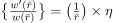 per unit of forecasted return. Flipping the sign delivers the headline formula
(11) 
A price increase lowers next year’s return forecast by percentage points. Dividing by converts this drop into an elasticity of returns, and multiplying by translates it into a demand elasticity.
We can now cleanly state the inelastic-markets result of Gabaix-Koijen. Start with the textbook prediction. Consider a mean-variance investor in a frictionless model where the dividend yield is and the long-run average return is . The predicted belief drag is  . This change in next year’s return forecast represents roughly
  of the average return forecast. With
  , this return elasticity translates to a
  change in demand. For the market as a whole, and
  , so
, so  . For an individual stock,
  and
and  , giving a demand elasticity that is one turn higher,
  . Gabaix-Koijen estimate an aggregate demand elasticity of
  . The textbook prediction is off by two orders of magnitude,
  !
!
Trailing PE Ratio
Sell-side analysts typically describe setting one-year-ahead price targets using a two-step process. First, an analyst forecasts the stock’s EPS over the next year based on non-price information. Then, the analyst capitalizes this short-term earnings forecast into a price target using the company’s current multiple,  , which is known as the trailing PE ratio
(12) ![\begin{equation*}\mathbb{F}_t[\mathrm{Price}_{t+1}] = \mathbb{F}_t[\mathrm{EPS}_{t+1}] \times \mathrm{PE}_t\end{equation*}](https://alexchinco.com/wp-content/ql-cache/quicklatex.com-70b551899765b82e3303734a47c4b3fc_l3.svg "Rendered by QuickLaTeX.com")
This price forecast implies that next year’s return forecast will consist of two components: the firm’s anticipated dividend yield and forecasted earnings growth
(13) ![\begin{align*}\mathbb{F}_t[\mathrm{Ret}_{t+1}] \;&=\; \bigg(\frac{\mathbb{F}_t[\mathrm{Div}_{t+1}]}{\mathrm{Price}_t}\bigg) \,+\, \bigg(\frac{\mathbb{F}_t[\mathrm{Price}_{t+1}] - \mathrm{Price}_t}{\mathrm{Price}_t}\bigg) \\ &=\; \bigg(\frac{\mathbb{F}_t[\mathrm{Div}_{t+1}]}{\mathrm{Price}_t}\bigg) \,+\, \bigg(\frac{\mathbb{F}_t[\mathrm{EPS}_{t+1}] {\times} \mathrm{PE}_t - \mathrm{EPS}_t {\times} \mathrm{PE}_t}{\mathrm{EPS}_t {\times} \mathrm{PE}_t}\bigg) \\ &=\; \bigg(\frac{\mathbb{F}_t[\mathrm{Div}_{t+1}]}{\mathrm{Price}_t}\bigg) \,+\, \bigg(\frac{\mathbb{F}_t[\mathrm{EPS}_{t+1}] - \mathrm{EPS}_t}{\mathrm{EPS}_t}\bigg)\end{align*}](https://alexchinco.com/wp-content/ql-cache/quicklatex.com-067b21fdb9767421b5580af9e40d65bf_l3.svg "Rendered by QuickLaTeX.com")
Since the analyst uses today’s PE ratio to forecast next year’s price, the multiple drops out of the price appreciation term. Regardless of the current level, the analyst anticipates that the firm’s price will grow at the same rate as its earnings.
Notice that only one of the two components of the analyst’s return forecast includes the current price. This is clearly going to have implications for demand elasticities. To see what those are, let’s look at a concrete example. Consider a company that realized earnings of  last year. Over the next year, analysts anticipate that the company’s earnings will grow by
  to
to ![\mathbb{F}_t[\mathrm{EPS}_{t+1}] = \mathdollar 5.035/\mathrm{sh}](https://alexchinco.com/wp-content/ql-cache/quicklatex.com-535d2b58ca7cf2c03ff969391f85e788_l3.svg "Rendered by QuickLaTeX.com") . The stock starts out trading at
. The stock starts out trading at  , giving the firm a trailing multiple of
  . Given how the market is currently pricing the company’s earnings, analysts expect the firm to be trading at a price of
 ![\mathbb{F}_t[\mathrm{Price}_{t+1}] = \mathdollar 5.035/\mathrm{sh} \times 20 = \mathdollar 100.70/\mathrm{sh}](https://alexchinco.com/wp-content/ql-cache/quicklatex.com-5085eb4ef709b92339020d76642bd4b4_l3.svg "Rendered by QuickLaTeX.com") next year. The company has committed to paying
next year. The company has committed to paying  in dividends next year, giving the firm an anticipated dividend yield of
  and a return forecast of
 ![\mathbb{F}_t[\mathrm{Ret}_{t+1}] = 0.7\% + 3.7\% = 4.4\%](https://alexchinco.com/wp-content/ql-cache/quicklatex.com-15fb95472b64834656ef545dbf1bb7b0_l3.svg "Rendered by QuickLaTeX.com") .
.
Now, imagine that the company’s current price suddenly increases by to  . The firm’s earnings over the last twelve months don’t move, . Nothing about the company’s fundamentals change, either. Analysts still have the same next-twelve-month earnings forecast, . But the company’s higher current price means that this short-term forecast will get capitalized at a higher multiple,
  , when setting a price target,
 ![\mathbb{F}_t[\mathrm{Price}_{t+1}] = \mathdollar 5.035/\mathrm{sh} \times 20.2 = \mathdollar 101.71/\mathrm{sh}](https://alexchinco.com/wp-content/ql-cache/quicklatex.com-ccd9417cbd9c450ac846415c6767a6b9_l3.svg "Rendered by QuickLaTeX.com") . Yet the higher price target has no impact on analysts’ beliefs about future price growth because the current earnings are also being priced using a multiple that is
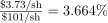
. Yet the higher price target has no impact on analysts’ beliefs about future price growth because the current earnings are also being priced using a multiple that is  higher. The higher current price level only affects analysts’ return forecast for next year by diluting the dividend yield. Instead of
  , analysts now anticipate a dividend yield of
  .
.
Prior to the price increase, the company’s forecasted payout was the  target price plus the forecasted dividend, which came out to
  total. The resale price contributed
 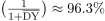 of the total payout. Following the unilateral price increase, the company’s multiple expanded and its price target also rose by . But its dividend forecast stood still. Hence, analysts’ forecasted payout didn’t rise by a full . The drag on analysts’ beliefs is thus
(14) 
This drag gets compared to the same average forecast as before, . But, given the much smaller starting value,  vs
vs  , the resulting elasticity of returns is much smaller,
  rather than
  . Assuming , you get a single-stock demand elasticity of
  and an aggregate demand elasticity of .
The trailing-PE approach gets you from down to  . The remaining distance, from down to the estimated , is likely due to rather than beliefs. Mandates, inertia, and the other demand-side frictions at the center of the inelastic-markets literature all mute the position response, which corresponds to
  . An
. An  closes the gap. On this reading, the trailing-PE rule and demand-side frictions are complements, not competitors. Beliefs deliver the first factor of
  . Frictions deliver the last factor of
  .
.
Learning Story
The trailing-PE rule hardcodes the link between this year’s multiple and next year’s multiple. A learning story can deliver something similar without hardcoding anything. Think about Grossman-Stiglitz. When the current price goes up by , an investor might worry that everyone else knows something she doesn’t. And, as a result, she might raise her forecast of the future payout. This is the story in Bastianello (2026).
Consider an investor who solves the following Gaussian inference problem. The investor has prior beliefs about the stock’s future payout
(15) 
For clarity, I’ve suppressed a constant term, which reflects discounting and the risk premium. I’ve also normalized the prior variance to  . The current price level is a noisy signal about the future payout
(16) 
 is the precision of the price signal. A larger value of
  implies that prices are more informative about the stock’s likely payout next year.
Standard Gaussian-updating rules imply that the investor’s posterior beliefs about the payout will be a weighted average
(17) ![\begin{equation*}\mathbb{E}_t[\log \mathrm{Payout}_{t+1}|\log \mathrm{Price}_t] \;=\; (1 {-} \lambda) \cdot \log \mathrm{Prior}_t \,+\, \lambda \cdot \log \mathrm{Price}_t\end{equation*}](https://alexchinco.com/wp-content/ql-cache/quicklatex.com-0f40570da89b78a75e33be679afdf4af_l3.svg "Rendered by QuickLaTeX.com")
Her beliefs are a true conditional expectation, so I write them with rather than . The weights reflect the precision of the price signal. The investor leans more heavily on the current price when it is a more precise signal about the stock’s future payout,  .
.
From here, it’s straightforward to derive the key inputs to the demand-elasticity formula. Start with the belief drag. Differentiating the log expected payout with respect to gives
(18) ![\begin{equation*}\frac{\partial \log \mathbb{E}_t[\mathrm{Payout}_{t+1}|\log \mathrm{Price}_t]}{\partial \log \mathrm{Price}_t} \;=\; \lambda \qquad \rightsquigarrow \qquad \mu \;=\; (1 {+} \overline{\mathrm{DY}}) \cdot (1 {-} \lambda)\end{equation*}](https://alexchinco.com/wp-content/ql-cache/quicklatex.com-c3e9e00a81b71437642624d587a27a5e_l3.svg "Rendered by QuickLaTeX.com")
Learning scales the entire textbook drag down by a factor of  . There’s no impact on how this drag gets converted into a return elasticity. For the market as a whole, we get a predicted demand elasticity of
(19) 
If the price signal is entirely uninformative,  , you get back the original formula. If the price signal is perfectly revealing,
  , the entire belief channel dies. Only the rebalancing term remains.
Partial Symmetry
I motivated the learning story above by pointing out that, if you squint, it looks a bit like the trailing-PE approach. In both cases, an investor sees the current price level change and assumes that most of the change will propagate into the future payout. Using a trailing PE is kind of like viewing the current price level as a very precise signal about the future payout.
Consistent with this intuition, it’s possible to make the two mechanisms produce identical elasticities. All you have to do is equate the belief drags. The trailing-PE approach says  . The learning story says
  . For both to produce the same value, you need
(20) 
Assuming would imply that  . A learner who put
  weight on the current price signal would have the same demand curve as an analyst who set price targets using a trailing PE,
  for a single stock and for the aggregate at . So there is a precise sense in which using a trailing PE and putting a lot of weight on the current price level are symmetric.
Gabaix-Koijen estimates . To match that result, a learning story would need to put weight on the current price of  or higher. This is worth pausing on. The learning model in Bastianello is built from standard Bayesian ingredients. The paper never talks in terms of trailing multiples. Yet at the weight implied by the data, the investor submits the same demand curve as an analyst using a trailing PE ratio. Fit to the data, the learning story does not offer an alternative to the trailing-PE mechanism. It approximates it.
But the symmetry isn’t perfect. And the way that it breaks is interesting. The key thing in the trailing-PE story is not the trailing PE. It is that the investor treats next period’s EPS forecast and the current price as unrelated. There is no present-value calculation connecting the two. Her EPS forecast comes from sales and margins, her level comes from the market, and neither number is evidence about the other.
The difference shows up in how a price shift reaches each investor. For the trailing-PE analyst, a rise in the current price level moves her price target by the same . So the capital-gain piece of her forecasted return never budges. The entire impact of the price shock arrives through the stock’s dividend yield, and that is why her drag equals  exactly.
By contrast, an investor who learns about the stock’s future payout from its current price sees both components of her payout forecast change. The price rise is news about fundamentals, which affects her beliefs about next year’s dividend and next year’s resale price. In this scenario, the investor’s belief drag gets spread across the whole forecast rather than concentrated in the dividend.
The apportionment can be made exact. At  , both investors mark up their payout forecast by
  in response to a price increase, leaving the same
  shortfall. But the two stories aren’t equivalent. They each place that gap in different places. The trailing-PE analyst increases her price target by . Her dividend-yield forecast absorbs the entire shortfall. The learner pins
  on the capital gain and
  on the dividend yield. In the running example, both investors would forecast the same payout next year,
  . The analyst gets there as
  . The learner gets there as
  . Same number, different tickets, and the dividend line is the tell.