1. Motivation
Imagine you’re a financial economist who thinks that some risk factor, , explains the cross-section of expected returns. And, you decide to test your hunch. First, you regress the realized returns of
  different assets on to estimate each asset’s exposure to the risk factor,
  :
:

Then, you regress these same assets’ average returns on their exposures the risk factor, :
![\begin{equation*} \mathrm{E} [ r_n ] = \hat{\alpha} + \hat{\lambda} \cdot \tilde{b}_n + \hat{\epsilon}_n \qquad n = 1, \, \ldots, \, N \end{equation*}](https://alexchinco.com/wp-content/ql-cache/quicklatex.com-e3d478cfa123a567c9c60758b2502ad5_l3.svg "Rendered by QuickLaTeX.com")
If is a priced factor, then the slope coefficient,  , should be large and the intercept,
  , should be zero.
This two-stage methodology dates back to Fama and MacBeth (1973). And, in keeping with the original paper, many financial economists still use a small set of portfolios as the assets in their empirical analysis. For example, Fama and French (1993) use  portfolios created by sorting stocks based on size and book-to-market. In theory, this is fine. If you’ve found a priced risk factor, then exposure to should affect the average returns of all assets. There is no theoretical guidance about which assets to use.
But, here’s the thing: econometrically, the number of assets has to matter. We live in a world with lots of factors to choose from. This is the “anomaly zoo” coined in Cochrane (2011). If you consider a model with more risk factors than you have assets  , then of course you can perfectly fit the data:
![\begin{equation*} \mathrm{E} [ r_n ] = 0 + {\textstyle \sum_{f \in \mathcal{K}}} \, \hat{\lambda}_f \cdot \tilde{b}_{n,f} + 0 \qquad n = 1, \, \ldots, \, N \leq K \end{equation*}](https://alexchinco.com/wp-content/ql-cache/quicklatex.com-e65fea1efdc49012638f9a71638edcbf_l3.svg "Rendered by QuickLaTeX.com")
After all, a system of linear equations with  unknowns is guaranteed to have a solution if .
Clearly, you need at least assets to test a -factor model. This is obvious. But, you can elaborate on this idea and say something useful in the related setting where  . This post answers the question: how many assets do you need when testing a
  -factor model chosen in a world with
  candidate factors?
2. Problem Formulation
Suppose we live in a world with assets and  candidate factors. Think about (McLean and Pontiff; 2016),
  (Harvey, Liu, and Zhu; 2016), or
  (Hou, Xue, and Zhang; 2017). We are looking for the asset-pricing model with the fewest factors that perfectly explains the cross-section of expected returns:
(★) ![\begin{equation*} \min_{\mathcal{K} \subseteq \mathcal{F}} \left\{ \, {\textstyle \sum_{f \in \mathcal{K}}} \, 1_{\{\hat{\lambda}_f \neq 0\}} \quad \text{s.t.} \quad \mathrm{E}[ r_n ] = {\textstyle \sum_{f \in \mathcal{K}}} \, \hat{\lambda}_f \cdot \tilde{b}_{n,f} \, \right\} \end{equation*}](https://alexchinco.com/wp-content/ql-cache/quicklatex.com-8ca5044b224bfe229258045fc8e92f0e_l3.svg "Rendered by QuickLaTeX.com")
This is just a mathematical way of applying Occam’s razor to our model-selection problem.
Here’s what I want to know: if we find a solution to this problem,  , how likely is it that is the only solution? In other words, if we find a
  -factor model that solves Problem (★) and perfectly explains the cross-section of expected returns, should we celebrate or slow clap? Have we found the simplest model of the world? Or, is this just one of many such -factor models that we were bound to uncover?
3. Similar Exposures
It turns out that the answer to this question is going to critically depend on the similarity of the assets’ exposures to the risk factors. To see why, just think about a world where  contains two copies of some risk factor in . Clearly, can’t be a unique solution to Problem (★) because you could just switch out the risk factor for its twin and have another -factor model explaining the cross-section of expected returns.
Donoho and Huo (2001) gives a nice way of generalizing this notion of similarity to situations where doesn’t contain multiple copies of the same factor. Specifically, they define the idea of mutual coherence:

Roughly speaking, you should think about mutual coherence as measuring the maximum correlation between the assets’ exposures to any pair of risk factors in . A large value of  , means that the assets have really similar exposures to some pair of risk factors in . And, in the extreme case where contains two exact copies of the same risk factor, we have
  . By contrast,
  if there are more assets than risk factors and the risk factors were independent.
But, since we are thinking about a world where there are more candidate risk factors than assets  , we know that
  . Even if the factors really are independent, some of them are going to have to look correlated in such a small sample. And, Welch (1974) characterizes exactly how correlated they will look:
(W) 
4. Theoretical Minimum
Now, we can answer our original question: when can we be sure that a solution to Problem (★) is unique? i.e., if we find a -factor model that perfectly explains the cross-section of returns for assets, should we be surprised? Donoho and Elad (2003) show that, if is a solution to Problem (★) and
(DE) 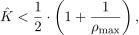
then is a unique solution. There are no other factor models that explain the cross-section of expected returns using or fewer factors. Inserting the bound from Equation (W) into the bound from Equation (DE) and then solving for yields:

What’s this equation telling us? Suppose we find a -factor model that perfectly explains the cross-section of expected returns—i.e., a factor model that solves Problem (★). If our empirical analysis used at least  assets, then we can be sure that we’ve found the simplest possible model. Whereas, if we only used
  assets, then there might be another asset-pricing model with the same number of factors that perfectly explains the cross-section of expected returns.
5. Plugging in Numbers
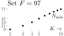 Let’s plug in some numbers to see if our formula for makes any sense. Here’s the first exercise. Suppose that there really are only
  candidate risk factors like in McLean and Pontiff (2016). The figure to the right plots the minimum number of assets we’d need to include in our empirical analysis (y-axis) to identify a model with factors (x-axis). We need to study at least
  assets to be sure that we’ve found a unique
  -factor model; we need to study at least
  assets to be sure that we’ve found a unique
  -factor model; and, we need to study at least
  assets to be sure that we’ve found a unique -factor model. This is an interesting exercise because it says that we shouldn’t be surprised if someone found a -factor model that perfectly explained the cross-section of expected returns for the
  size- and value-sorted portfolios used in Fama and French (1993). In other words, since Gene and Ken already claimed the first factors, we can’t do cross-sectional asset pricing tests with just the Fama and French (1993) portfolios any more. Even if we found a -factor model that perfectly explained the cross-section of expected returns, there’d be no guarantee that it’d be unique.
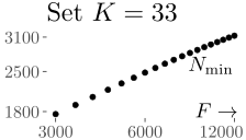 Now, let’s consider a second exercise. In a recent NBER working paper, Kozak, Nagel, and Santosh (2017) found used a machine-learning rule to identify a cross-sectional asset-pricing model with
  factors. For the sake of argument, let’s imagine that this
  -factor model perfectly explained the cross-section of expected returns. The figure to the left plots the minimum number of assets they’d need to include in their empirical analysis (y-axis) to be sure that they’d found the only such -factor model in a world with candidate factors (x-axis). There are roughly
  stocks at the moment. So, if their -factor model had perfectly explained the cross-section of expected returns, then you should be really excited by this result if you think there are less than
  candidate factors.
Let’s do one last exercise before we call it quits. Notice that, as the number of candidate factors gets large, the minimum number of assets we’d need to identify a -factor model only depends on :
(1) 
This observation is cool because, by setting  and solving for , we can compute the size of the most complicated factor model that we can estimate with stocks is
  . No matter how many candidate factors there are, if we find a -factor model that perfectly explains the cross-section of expected returns, then we know it is unique if we use the universe of all stocks in our empirical analysis.
 , and there are
  noise traders present in this market. And, assume that this price is a linear function of three variables:
 denotes noise due to the madness of crowds, and
  denotes noise due to random supply shocks. The negative sign on supply noise comes from the fact that more supply means lower prices. You can think about the supply noise as the result of
  noise traders, and each individual trader in this crowd has demand that’s iid normal:

 , is a normally distributed signal about the aggregate demand coming from the crowd of noise traders:
 , it must be because either the crowd of noise traders has high demand,
  , or there is unexpectedly low supply,
  . The question I want to answer below is: how hard is it for traders to figure out which noise source is responsible?
 . So, if we knew the distribution of the number of noise traders in the market, then we could evaluate the remaining integral and solve for the most likely value for the crowd’s aggregate demand given the observed pricing error:
 , is governed by the following stochastic differential equation:
 denotes the rate at which the crowd of noise traders grows,
  denotes the rate at which noise traders lose interest,
  is a Wiener process capturing random fluctuations in the number of noise traders in the crowd, and
  denotes the volatility of these random fluctuations.
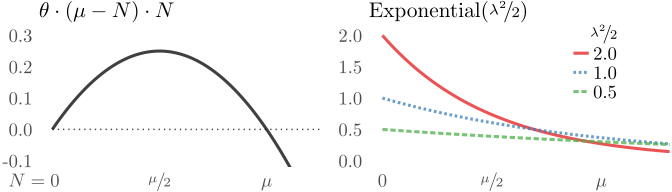
 , is a quadratic function of the number of noise traders as shown in the figure below. This nonlinearity is what allows the model to generate population booms and busts. This nonlinearity will occur if existing noise traders try to recruit their friends to enter the market as well (see
  denotes the typical number of noise traders that could potentially be persuaded to join the crowd. And,
  captures the intensity with which existing noise traders persuade their remaining
  friends to join.
 .
.
 and
and  . If
. If  . To see why, think about how the system behaves as the crowd size gets small. When
  , the crowd grows at an almost linear rate,
  . So,
. So,  . By contrast, if the growth rate is larger than the rate of decay when
  , then we will find that number of noise traders in the crowd will be governed by an
  :
:
 reveals that the rate parameter will be largest as
  —i.e., when the growth rate is barely larger than the decay rate when the crowd size is small. Makes sense.
 . It turns out that, if the variance of the crowd’s aggregate demand is drawn from an Exponential distribution, then it’s easy to solve the integral in Equation (
 , then the optimization problem in Equation (
 (see
(see 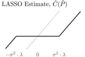 There’s something weird about this result, though. Using the LASSO implies that:
 if
if  and
and  . So, if the observed pricing error is relatively small,
  , then a fully-rational trader will walk away from the market believing that
  . He will completely neglect the risk coming from the crowd of noise traders.
 ) when either the crowd of noise traders tends to be smaller (
 is larger). And, this basic intuition should carry over to other situations where the size of the crowd of noise traders has some other fat-tailed distribution rather than an Exponential distribution.
 , in future periods
  And, suppose that there’s a unit mass of small agents,
 ![i \in (0, \, 1]](https://alexchinco.com/wp-content/ql-cache/quicklatex.com-16436c8e931ed16f2a870b07e315509e_l3.svg "Rendered by QuickLaTeX.com") , who have noisy priors about these dividends,
, who have noisy priors about these dividends,
 . This assumption means that, by aggregating agents’ demand, equilibrium prices can contain information about dividends that isn’t known by any individual agent.
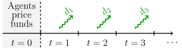 This unit mass of agents is split into two different groups: long-term investors and short-run traders. At time
  , each group of agents trades shares in its own separate fund,
  , that offers frequency-specific exposure to the company’s dividends at times
  . The long-term investors,
 ![i \in (0, \, \sfrac{1}{2}]](https://alexchinco.com/wp-content/ql-cache/quicklatex.com-f9cd6ec14723d24913ac9820a3cd2652_l3.svg "Rendered by QuickLaTeX.com") , trade the low-frequency fund which has a payout:
, trade the low-frequency fund which has a payout:
![i \in (\sfrac{1}{2}, \, 1]](https://alexchinco.com/wp-content/ql-cache/quicklatex.com-5444575605cdfca9b310c48c1e7b86d2_l3.svg "Rendered by QuickLaTeX.com") , trade the high-frequency fund which has a payout:
, trade the high-frequency fund which has a payout:
 , and then chooses the number of shares to buy,
  , in order to maximize his expected utility at the end of time
  :
:![\begin{equation*} \max_{x_f^{(i)}} \mathrm{E}^{(i)}\left[ \, - e^{ \, - \alpha \cdot \{d_f - p_f\} \cdot x_f^{(i)} \, } \, \middle| \, p_f \, \right] \quad \text{for some} \quad \alpha > 0 \end{equation*}](https://alexchinco.com/wp-content/ql-cache/quicklatex.com-73ae822cb250c86fc903e846e0687a39_l3.svg "Rendered by QuickLaTeX.com")
![\mathrm{E}^{(i)}[\cdot|p_f]](https://alexchinco.com/wp-content/ql-cache/quicklatex.com-7a88f40831c34e3bf0571b8a460837f4_l3.svg "Rendered by QuickLaTeX.com") denotes agent
denotes agent  ‘s conditional expectation, and
  denotes his risk-aversion parameter.
 denote the number of shares of the company’s stock that are available for purchase at time
  . We say that “markets clear” at time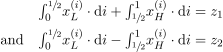
 and
and  denote the number of available shares at each frequency.
![\mathrm{X}(\mathrm{E}^{(i)}[d_f|p_f], \, p_f) = x_f^{(i)}](https://alexchinco.com/wp-content/ql-cache/quicklatex.com-c63f920499536e093da9aaa25f966997_l3.svg "Rendered by QuickLaTeX.com") , and a price function,
, and a price function,  , such that
  by studying its equilibrium price at time
 to update their time
  and
and  to denote aggregate demand: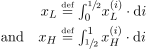
 to every one of its shareholders, the low-frequency fund has to buy
  . And, to deliver
  to every one of its shareholders, the high-frequency fund has to buy
  shares between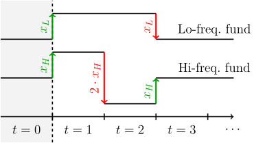
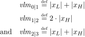
 , because short-run traders don’t get any new information after time
 , which represents the
  . And, with normally-distributed signals, we
  after seeing
 ![\begin{equation*} \mathrm{E}^{(i)}[d_f|p_f] = {\textstyle \left\{ \frac{1}{1 + \mathit{SNR}}\right\}} \cdot \mu_f^{(i)} + {\textstyle \left\{ \frac{\mathit{SNR}}{1 + \mathit{SNR}}\right\}} \cdot p_f \end{equation*}](https://alexchinco.com/wp-content/ql-cache/quicklatex.com-4a178e548d97f55763a718b17ee25deb_l3.svg "Rendered by QuickLaTeX.com")
 denotes agent
  or
or  . And, we can then use these posterior beliefs to compute agents’ equilibrium demand rule by
 ![\begin{equation*} \mathrm{X}(\mathrm{E}^{(i)}[d_f|p_f], \, p_f) = \{1 + \mathit{SNR}\} \cdot {\textstyle \big\{ \frac{\mathrm{E}^{(i)}[d_f|p_f] - p_f}{\sigma} \big\}} \cdot {\textstyle \big\{ \frac{1}{\alpha \cdot \sigma} \big\}} \end{equation*}](https://alexchinco.com/wp-content/ql-cache/quicklatex.com-b0c32001e4acdfaab6b73edfd28be821_l3.svg "Rendered by QuickLaTeX.com")

 . In other words, fund prices at time
  small).
 . And, from Equation (
 :
:
![\mathrm{Cov}[d_2, \, d_H] = - \,\sigma^2](https://alexchinco.com/wp-content/ql-cache/quicklatex.com-5ee8d116a7c42f264689d17d2696d5fc_l3.svg "Rendered by QuickLaTeX.com") .
. denote their demand at time
  , and a large dividend payout at time
  , they know that
  is likely small. And, as a result, they’ll short more shares at time
  . By contrast, when they observe a high price for the low-frequency asset at time
  , they know that
  .
. is unchanged and:
 .
. variables:
 denotes the mean return, and each
  captures the relationship between returns and the
  th right-hand-side variable. Some notation: I’m going to be using a “star” to denote true parameter values and a “hat” to denote in-sample estimates of these values. e.g.,
  denotes an in-sample estimate of
  ,
,  ,
,  , and
, and  .
.

 is homework question from Econometrics 101. Nothing could be simpler.
![\begin{align*} \min_{\alpha, \, \beta_1, \, \ldots, \, \beta_V} \left\{ \, {\textstyle \frac{1}{S}} \cdot {\textstyle \sum_s} \, \left( r_s - [\alpha + {\textstyle \sum_v} \, \beta_v \cdot x_{s,v}] \right)^2 \, \right\}, \end{align*}](https://alexchinco.com/wp-content/ql-cache/quicklatex.com-6d99e55beb9f5f542c09f807e7d9d594_l3.svg "Rendered by QuickLaTeX.com")
 right-hand-side variable, then
  the best predictions come from using
  . But, it turns out that when there’s
  we can make better predictions with less likely parameters. When
  , this is just
![\begin{align*} - \, \log \mathrm{Pr}(\mathbf{r} | \{\alpha, \, \beta_1, \, \ldots, \, \beta_V\}) &= {\textstyle \frac{1}{2 \cdot (S \cdot \sigma^2)}} \cdot {\textstyle \sum_s} \left(r_s - [\alpha + {\textstyle \sum_v} \, \beta_v \cdot x_{s,v}] \right)^2 + \cdots \end{align*}](https://alexchinco.com/wp-content/ql-cache/quicklatex.com-3cdacf38667dabb31ae4f354544b1eee_l3.svg "Rendered by QuickLaTeX.com")
 ” at the end denotes a bunch of terms that don’t include any of the parameters that we’re optimization over. Optimizing each parameter value then gives the
 ![\begin{align*} 0 &= {\textstyle \frac{1}{S}} \cdot {\textstyle \sum_s} \left( r_s - [\hat{\alpha}^{\text{ML}} + {\textstyle \sum_v} \, \hat{\beta}_v^{\text{ML}} \cdot x_{s,v}] \right) \cdot 1 \\ \text{and} \quad 0 &= {\textstyle \frac{1}{S}} \cdot {\textstyle \sum_s} \left( r_s - [\hat{\alpha}^{\text{ML}} + {\textstyle \sum_v} \, \hat{\beta}_v^{\text{ML}} \cdot x_{s,v}] \right) \cdot x_{s,v} \quad \text{for each } v = 1, \, \ldots, \, V. \end{align*}](https://alexchinco.com/wp-content/ql-cache/quicklatex.com-d9d6ee58f1d5388b2d4c3da0bc01a5c6_l3.svg "Rendered by QuickLaTeX.com")
 equations and
 . With access to this oracle, we can compute our mean squared error when using the maximum-likelihood estimates to predict returns given any choice of true parameter values:
![\begin{align*} \mathrm{E} \left[ \, \left( r_s - [\hat{\alpha}^{\text{ML}} + {\textstyle \sum_v} \, \hat{\beta}_v^{\text{ML}} \cdot x_{s,v}] \right)^2 \, \middle| \, \{ \alpha^\star, \, \beta_1^\star, \, \ldots, \, \beta_V^\star \} \, \right] &= \sigma^2 + 1 \cdot (\sfrac{\sigma^2}{S}) + V \cdot (\sfrac{\sigma^2}{S}). \end{align*}](https://alexchinco.com/wp-content/ql-cache/quicklatex.com-d0f562d984883586791916a7e8f61469_l3.svg "Rendered by QuickLaTeX.com")
 . And, the second and third terms,
  and
and  , capture the
![\lambda \in [0, \, 1]](https://alexchinco.com/wp-content/ql-cache/quicklatex.com-719927087d350d9c027adaaf633d33bd_l3.svg "Rendered by QuickLaTeX.com") denotes a bias factor that
denotes a bias factor that  . So, with access to an oracle, we can compute our mean squared error when using the James-Stein estimates to predict returns just like before:
![\begin{align*} \mathrm{E} \left[ \, \left( r_s - [\hat{\alpha}^{\text{ML}} + {\textstyle \sum_v} \, \hat{\beta}_v^{\text{JS}} \cdot x_{s,v}] \right)^2 \, \middle| \, \{ \alpha^\star, \, \beta_1^\star, \, \ldots, \, \beta_V^\star \} \, \right] &= \sigma^2 + 1 \cdot (\sfrac{\sigma^2}{S}) \\ &\quad + V \cdot \left\{ \, (1 - \lambda)^2 \cdot (\sfrac{\sigma^2}{S}) + \lambda^2 \cdot ({\textstyle \frac{1}{V}} \cdot {\textstyle \sum_v} \, |\beta_v^\star|^2) \, \right\}. \end{align*}](https://alexchinco.com/wp-content/ql-cache/quicklatex.com-36e32a6a91a1608c7d11285e589d9463_l3.svg "Rendered by QuickLaTeX.com")
 and
and  , then using the most likely parameter values rather than the true parameter values to predict returns is going to cause less damage. But, bias is going to generate really bad predictions whenever the true parameter value is large
  . The
. The  and
and  terms capture these two opposing forces.
![\lambda \in (0, \, 1]](https://alexchinco.com/wp-content/ql-cache/quicklatex.com-8809687cecc74fe1171a83cf272a2b6e_l3.svg "Rendered by QuickLaTeX.com") such that:
such that:
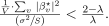
 right-hand-side variable. When there are
 ![\begin{align*} \lambda^\star &= \arg \min_{\lambda \in [0, \, 1]} \left\{ \, (1 - \lambda)^2 \cdot (\sfrac{\sigma^2}{S}) + \lambda^2 \cdot \left( {\textstyle \frac{1}{V}} \cdot {\textstyle \sum_v} \, |\beta_v^\star|^2 \right) \, \right\} \end{align*}](https://alexchinco.com/wp-content/ql-cache/quicklatex.com-ba2b47a4ed600cd9072cc775461e3bc0_l3.svg "Rendered by QuickLaTeX.com")
 :
:
 is close to
  ), then using the most likely parameter values rather than the true parameter values is going to increase our prediction error a lot. So, we should use more biased parameter estimates.
 on the left-hand side is a
 ![\begin{align*} \mathrm{E} \left[ \, \left( r_s - [\hat{\alpha}^{\text{ML}} + {\textstyle \sum_v} \, \hat{\beta}_v^{\text{ML}} \cdot x_{s,v}] \right)^2 \, \right] &= \sigma^2 + 1 \cdot (\sfrac{\sigma^2}{S}) + V \cdot (\sfrac{\sigma^2}{S}), \end{align*}](https://alexchinco.com/wp-content/ql-cache/quicklatex.com-decec2e5ac909130ab5adc9ec4882759_l3.svg "Rendered by QuickLaTeX.com")
 maximum-likelihood estimates can move independently. There is an adding-up constraint.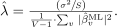
 only if
  . After all, if there’s only
  . With this estimated amount of bias, our prediction error becomes
![\begin{align*} \mathrm{E} \left[ \, \left( r_s - [\hat{\alpha}^{\text{ML}} + {\textstyle \sum_v} \, \hat{\beta}_v^{\text{JS}} \cdot x_{s,v}] \right)^2 \, \right] &= \sigma^2 + 1 \cdot (\sfrac{\sigma^2}{S}) + (1 - \lambda)^2 \cdot (\sfrac{\sigma^2}{S}), \end{align*}](https://alexchinco.com/wp-content/ql-cache/quicklatex.com-6fbfd084a5a865cfaa82b2e68e69e563_l3.svg "Rendered by QuickLaTeX.com")
 possible subsets of variables. And, this just isn’t feasible when
  .
. is the only candidate variable traders are considering, then it’s easy to use the
 and
and  . If the solution is some
  , then
  , then
  .
.
 . Thus, traders can’t take a strictly Bayesian approach to variable selection when there are lots of variables to choose from.

 and
and  , and see which one gives a smaller result. Practically speaking, this means running an OLS regression,
  , and checking whether or not the penalized residual variance,
  , is smaller than the raw return variance,
  .
. Most explanations for why (
 stocks and
  variables. The diagram above summarizes the correlation structure between these variables and returns. The red bar is the total variation in returns. The blue bars represent the portion of this variation that’s related to each of the
  and
and  are perfectly uncorrelated in-sample:
![\begin{align*} \widehat{\mathrm{Cor}}[x_1, \, x_2] &= 0. \end{align*}](https://alexchinco.com/wp-content/ql-cache/quicklatex.com-e2b3815a46bc46a944e1fbc606adbd44_l3.svg "Rendered by QuickLaTeX.com")
 :
:![\begin{align*} \widehat{\mathrm{Cor}}[x_1, \, x_3] = \widehat{\mathrm{Cor}}[x_2, \, x_3] &= 0.41. \end{align*}](https://alexchinco.com/wp-content/ql-cache/quicklatex.com-7fdd6fb9360b7b326633a81d896de148_l3.svg "Rendered by QuickLaTeX.com")
![\begin{align*} \widehat{\mathrm{Cor}}[r, \, x_1] = \widehat{\mathrm{Cor}}[r, \, x_2] &= 0.62 \\ \widehat{\mathrm{Cor}}[r, \, x_3] &= 0.67. \end{align*}](https://alexchinco.com/wp-content/ql-cache/quicklatex.com-5261763e891cc5750d0865b9b429f0c7_l3.svg "Rendered by QuickLaTeX.com")

 is actually the subset of variables that minimizes (

 . The problem is unavoidable in the real world where there are almost as many candidate variables as there are stocks because independent variables are still going to be correlated in finite samples.
 and
and  , the in-sample correlation between
  and
and  when
when  is roughly:
 , our estimates won’t be exactly zero in finite samples.
 is:
is:![\begin{align*} \mathrm{Pr}[ |\hat{\rho}_{v,v'}| > c ] &= 2 \cdot \mathrm{Pr}[ \hat{\rho}_{v,v'} > c ] = 2 \cdot \mathrm{\Phi}(c \cdot \!\sqrt{S}). \end{align*}](https://alexchinco.com/wp-content/ql-cache/quicklatex.com-c581a1f99fce1aa1b3a1ef168e290342_l3.svg "Rendered by QuickLaTeX.com")
 pairs of variables, we know that the probability that no pair has a correlation more extreme than
 ![\begin{align*} \mathrm{Pr}[ \max |\hat{\rho}_{v,v'}| \leq c ] &\leq \big( \, 1 - 2 \cdot \mathrm{\Phi}(c \cdot \!{\textstyle \sqrt{S}}) \, \big)^{\frac{1}{2} \cdot V^2}. \end{align*}](https://alexchinco.com/wp-content/ql-cache/quicklatex.com-220af27b62f366ff0ef0d1a2b0e3e964_l3.svg "Rendered by QuickLaTeX.com")
 shows up as an exponent in the equation above, the probability that all pairwise in-sample correlations happen to be really small is going to shrink exponentially fast as traders consider more and more variables. This means that finite-sample effects are always going to make evaluating (
 from the previous example might seem like an unreasonably high number for independent random variables, something that only happens when
  . But, the figure above shows that even when there are
  stocks, there’s still a
  chance of observing an in-sample correlation of at least
  when considering
  candidate variables.
 Market efficiency has been an
  even if none of the variables actually predicts returns. So, researchers have focused on correcting p-values.
![\begin{align*} \min_{{\boldsymbol \delta} \in \{0, \, 1\}^V} \left\{ \, {\textstyle \frac{1}{S}} \cdot {\textstyle \sum_s} (r_s - {\textstyle \sum_v} [\hat{\beta}_v^{\text{OLS}} \cdot x_{s,v}] \cdot \delta_v)^2 \quad \text{subject to} \quad k \geq {\textstyle \sum_v} \delta_v \, \right\}, \end{align*}](https://alexchinco.com/wp-content/ql-cache/quicklatex.com-62670743563fb449b0f38aeec78b91e8_l3.svg "Rendered by QuickLaTeX.com")
 variables that predicts returns is equivalent to finding the cheapest way to cover the red bar with blue bars at a cost of
  -bit passcode would involve a brute-force search over
  parameter values, which would take
  parameter values. We might be able to approximate it. But, the exact collection of variables may as well be in a vault somewhere.

You must be logged in to post a comment.