1. Motivation

This post looks at the consequences of ETF rebalancing. These funds follow pre-announced rules that involve discrete thresholds. The well-known SPDR tracks the S&P 500, but there are over 1400 different ETFs tracking a wide variety of different underlying indexes. When any of these underlying indexes change, the corresponding ETFs have to change their holdings. These thresholding rules mean that, in an extreme example, if Verisk Analytics gets larger and moves from being the st largest stock to being the th largest stock (actually happened), then the ETFs tracking the S&P 500 are going to suddenly have to build large positions in Verisk over a relatively short period of time. See here for more examples.

When there are many different ETFs tracking many different thresholds, these rebalancing rules can interact with one another and amplify small initial demand shocks. For example, when Verisk increases in size and gets bought by ETFs tracking the S&P 500, it will be slightly more correlated with the market (Barberis, Shleifer, and Wurgler, 2005). As a result, ETFs like SPHB that track large-cap high-beta stocks might have to buy Verisk as well, which in turn can have further consequences down the line. This is what journalists have in mind when they worry about ETFs “turning the market close into a buying or selling frenzy.” To model this phenomenon, I use an approach based on branching processes à la Nirei (2006).

The idea that traders might herd (Devenow and Welch, 1996) or amplify shocks (Veldkamp, 2006) is not new. But, these rebalancing rules can also transmit shocks to completely unrelated corners of the market. This idea is new. Rebalancing involves buying one stock and selling another. It sounds obvious, but it matters that we’re looking at “rebalancing” rules and not just “purchasing” rules. For instance, when Verisk got added to the S&P 500, it replaced Joy Global, a mining-tools manufacturing company. So, all of the ETFs tracking the S&P 500 had to sell their positions in Joy Global, pushing Joy’s price down and making it more likely that ETFs that need to hold a position in mining companies choose one of Joy’s competitors like ABB Limited. And, this additional demand for ABB can cause subsequent rebalancing, which is the result of an initial change in the value of Verisk, a totally unrelated stock.

No trader would ever be able to guess that the reason another Swiss company like Novartis is realizing selling pressure is that Verisk was Joy Global in the S&P 500, which caused ETFs tracking the S&P 500 to sell Joy, which caused other industrial ETFs to replace Joy with ABB Limited, which caused still other ETFs tracking the largest stocks in each European country to replace their positions in Novartis with a position in ABB. So, even though each ETF’s rebalancing rules are completely predictable, their aggregate behavior generates noise. By analogy, the population of France at any given instant is a definite fact. It is not random. No one is timing births by coin flips, dice rolls, radioactive decay, etc… But, as John Maynard Keynes pointed out, whether this number is even or odd at each instant is effectively random. Were or people born in Paris during the time it took you to finish counting the population of Nice?

2. Market Structure

Suppose there’s a single stock that can be held by different ETFs, and each fund’s demand for the stock, , is the sum of different components:

(1)  

When writing down models of the ETF market, people usually only think about the first component, . This is just the intrinsic demand that an ETF would have for the stock if it were the only fund in the market, like the SPDR was in the early 1990s. If there are no large-cap high-beta ETFs, then having the SPDR purchase additional shares of Verisk wouldn’t have any knock-on effects in the example above. Think about shocks to each fund’s as shocks to whether or not the stock is included in the fund’s benchmark index.

The second component, , captures how an ETF’s demand is affected by the decisions of other ETFs. This is the effect of S&P 500-tracking ETFs on the holdings of ETFs that track a large-cap high-beta index. Because buying by one ETF leads to additional buying by other ETFs, is increasing in ETF demand:

(2)  

Because each ETF’s demand only has a subtle effect on other ETFs’ demand, we have that:

(3)  

where is Landau notation. So, when there are more ETFs that might hold a stock, each ETF’s decisions have a smaller effect on the decisions of its peers. In the theoretical analysis below, I’m going to study the function , which satisfies this property.

Finally, the third component, , reflects the fact that ETFs use thresholding rules. Even if Verisk has a market capitalization that is smaller than the th largest stock, Verisk won’t be held by the SPDR, which tracks the S&P 500. The moment Verisk becomes the th largest stock, the SPDR is going to have to buy a large block of shares. This threshold-adjustment component is defined using modular arithmetic,

(4)  

where and is the remainder that’s left over after dividing by . So, if shares and an ETF would have bought shares, then and its resulting demand is shares. A fund is always demanding some multiple of shares. Think about as the size of a typical ETF’s adjustment once a stock is added to its benchmark.

3. Equilibrium Concept

What does it mean for this market to be in equilibrium, and how does the market transition between equilibria? Via Tarski’s fixed-point theorem, we know that for any choice of , if

1. both and are bounded, and
2. there are scalars and ,

then there exists a solution, , to Equation (1) for all funds. This solution is the equilibrium associated with . Here, and denote the upper and lower bounds on —i.e., ; and, and denote the upper and lower bounds on . To make things concrete, note that, if , then .

At the start of each trading day, the market is in an equilibrium at associated with the intrinsic demand . We can normalize this value to . Then, over the course of the day, the stock’s characteristics change. It gets added to some ETFs’ benchmarks. I model this as a shock to each ETF’s intrinsic demand,

(5)  

where is positive with mean and distributed i.i.d. across funds. This shock is divided through by so that its impact is the same magnitude as the feedback effect from one ETF’s demand to another. Given this shock, how will ETFs’ demand evolve over the course of the final to minutes of trading?

To answer this question, we need to define how ETFs update their demand. I follow the approach used in Cooper (1994) where ETFs adjust their positions by applying the best response function iteratively. In the first round, ETFs adjust their holdings by if they realize a sufficiently large shock to their intrinsic demand:

(6)  

Then, in each subsequent period, ETFs adjust their holdings by if the demand pressure from other ETFs is sufficiently large:

(7)  

This process continues until no more changes are required at . Initially, the shock is exogenous, ; then, in all later rounds the shock comes from other ETFs, . Importantly, ETFs in this model don’t proactively adjust their positions to account for future changes in demand that they see coming down the line in future iterations. After all, ETFs are constrained to mimic their benchmarks.

4. Cascade Length

It is now possible to show that small initial shocks to each ETF’s demand can lead to long rebalancing cascades. Let denote the number of ETFs that buy additional shares of the target stock in period :

(8)  

Similarly, let denote the total number of ETF position changes from time to time :

(9)  

So, when , then a small initial shock will cause a large number of ETFs to change their positions later on. This is what I mean by the length of a rebalancing cascade.

In order to characterize the distribution of analytically, I need to make a couple of functional form assumptions. First, I assume that the interaction of ETF-demand schedules is governed by the rule:

(10)  

with parameter . As gets larger and larger, each ETF’s demand has a larger and larger effect on other ETFs’ demand schedules. Finally, suppose that the distribution of ETF intrinsic demands,

(11)  

is uniformly distributed on the interval from to .

Using results from Harris (1963) it’s possible to show that, as the number of funds gets large, , the sequence of adjustments converges to a Poisson-distributed Galton-Watson process. The probability-density function for the total cascade length is given by:

(12)  

The figure above plots this function when and .

A Galton-Watson process, , is stochastic process that starts out with formula and then evolves according to the rule

(13)  

where is a set of i.i.d. Poisson-distributed random variables. To illustrate by example, the figure below displays a single realization from a Galton-Watson process. In this example, there are total ETFs that rebalance their holdings in response to an initial demand shock. In this example, the rebalancing cascade lasts rounds. There are ETFs that rebalance in the second round, and the rebalancing demand from the third of these ETFs causes two more ETFs to adjust their positions, .

Given the probability-density function described above, it’s easy to show that the mean and variance of the number of ETFs that rebalance is:

(14)  

So, even when each individual ETF realizes a shock to its intrinsic demand over the course of the trading day that is quite small on average, , the stock can still realize large demand shocks when each ETF’s demand has a large spillover effect, , and when they don’t have to make very granular position changes, . This is the amplification result I mentioned above. The figures below verifies these calculations using simulations with ETFS. In particular, the left panel shows that the initial shock of only leads to more than one rebalancing cascade on average when .

1. Introduction

There are many reasons why two houses might have different prices. To start with, one house might just be larger or have a better layout than the other. Let’s call these sorts of house-to-house differences “fine-grained”. But, prices can also vary for reasons that have nothing to do with the houses themselves. Even if two houses are physically identical, one house might sit in a more attractive neighborhood or belong to a better school district. Let’s call such differences over larger scales “coarse-grained”.

Different scales dominate in different places. In some counties, most of the price variation comes from fine-grained, house-to-house differences. Think about Los Angeles, CA where there is a lot of heterogeneity in the age and quality of the housing stock, even for houses that are right next door to one another. But, there are also coarse-grained counties where most of the house-price variation occurs over much larger scales. Think about Orange County, CA where the typical house is part of a subdivision. While there are lots of differences between subdivisions in Orange County, all the houses within each subdivision are typically built in a similar style by a single company at the exact same time.

This post shows how to estimate the characteristic scale of house-price variation in a county. That is, it shows how to tell if a county is fine-grained like Los Angeles, coarse-grained like Orange County, or somewhere in between. To do this, I introduce a new scale-specific variance estimator based on the Allan variance. This estimator decomposes the cross-sectional house-price variation in a given county into scale-specific components such as the amount of variation that arises from comparing randomly selected houses or the amount of variation that arises from comparing randomly selected neighborhoods.

Why not just compare the variance of the individual house prices to the variance of the neighborhood-level averages? The answer is simple: those calculations aren’t independent. Fine-grained counties with lots of house-to-house variation will mechanically have more variance in their average neighborhood-level prices. Just imagine the extreme case where all of the variation comes from house-to-house differences and each house’s price is independently drawn from the same normal distribution, . In a world where the th neighborhood has houses, the variance of the neighborhood-level average price, , would be increasing in the amount of house-to-house variation, . I use this new scale-specific estimator because I don’t want to confuse these sorts of emergent neighborhood-level fluctuations with the honest-to-goodness neighborhood-level differences.

2. Data-Generating Process

Consider a county with houses and neighborhoods where there are houses in each neighborhood so that . Suppose that house prices are the sum of a neighborhood-level value and a house-level value,

(1)  

with and . Think about neighborhood-level values as the quality of the local school district or the attractiveness of the nearby restaurant scene. This value is coarse-grained. You can have a mansion or a hovel in a nice school district. The house-level value, by contrast, relates to the characteristics of each particular house. This value is fine-grained.

Given this data-generating process, we know that a fraction

(2)  

of the variation in house prices comes from neighborhood-level differences. This is the object of interest in the current post. If is close to , then the county is dominated by coarse-grained variation in house prices and looks like Orange County, CA. If is close to , then the county is dominated by fine-grained variation in house prices and looks more like Los Angeles, CA. In the analysis below, I’m going to show how to estimate in simulated data.

3. Naïve Estimate of λ

One way to estimate would be to look at a variance ratio. You might first compute the average price in each neighborhood,

(3)  

and then look at the ratio of the variance of the neighborhood-level average prices to the total house-price variance:

(4)  

The thought process behind this calculation is really simple. If different neighborhoods have very different prices, then there should be a lot of variation in the average neighborhood-level price. In fact, it turns out to be too simple. While it is true that this naïve calculation will generate a higher in counties with lots of coarse-grained neighborhood-level variation, it will also be high in counties with lots of fine-grained house-to-house variation.

To see why, let’s look at the variance of the average price in each county:

(5)  

This variance consists of parts: the true neighborhood-level variance, ; differences in neighborhood-level prices from fine-grained variation, ; and, a correction for the unknown sample mean, . If we solve for the true amount of neighborhood-level variation,

(6)  

we see that it’s going to be smaller than the variation in neighborhood-level average prices. Counties with lots of fine-grained, house-to-house differences look like they have too much neighborhood-level house-price variation. What’s more, in the simulations plotted below [code] where the county has houses, you can see that the nature of this bias is going to vary in a non-trivial way as the number of neighborhoods and the amount of coarse-grained, neighborhood-level variation changes.

4. Corrected Estimate of λ

In order to fix the problem, we need a way of simultaneously estimating neighborhood-level and house-level price variation and then using the second estimate to correct the bias in the first. It turns out that you can do this by running a simple cross-sectional regression,

(7)  

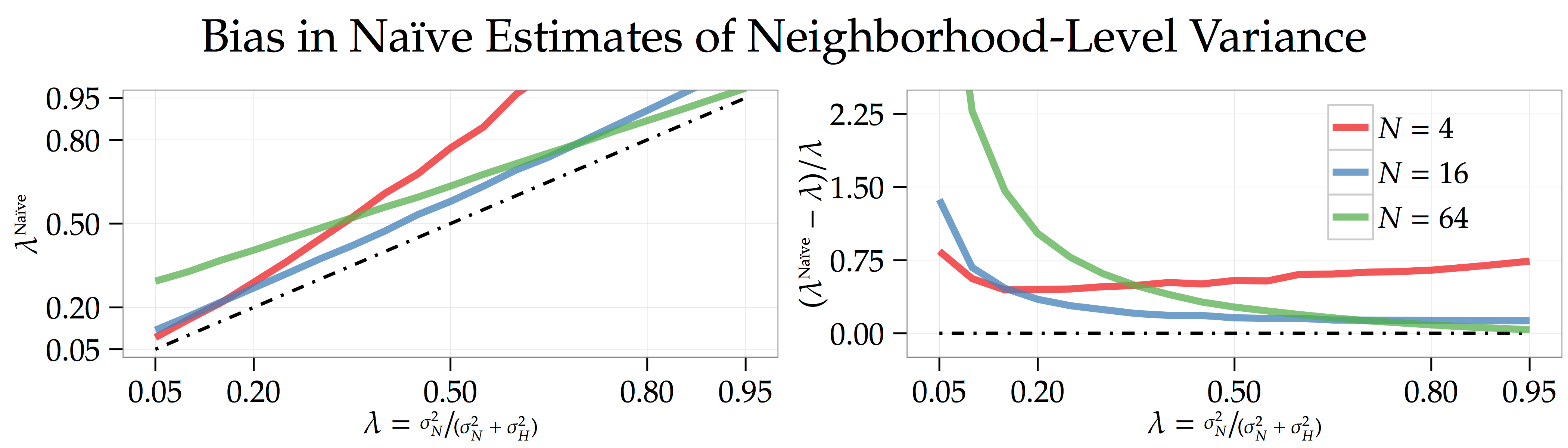
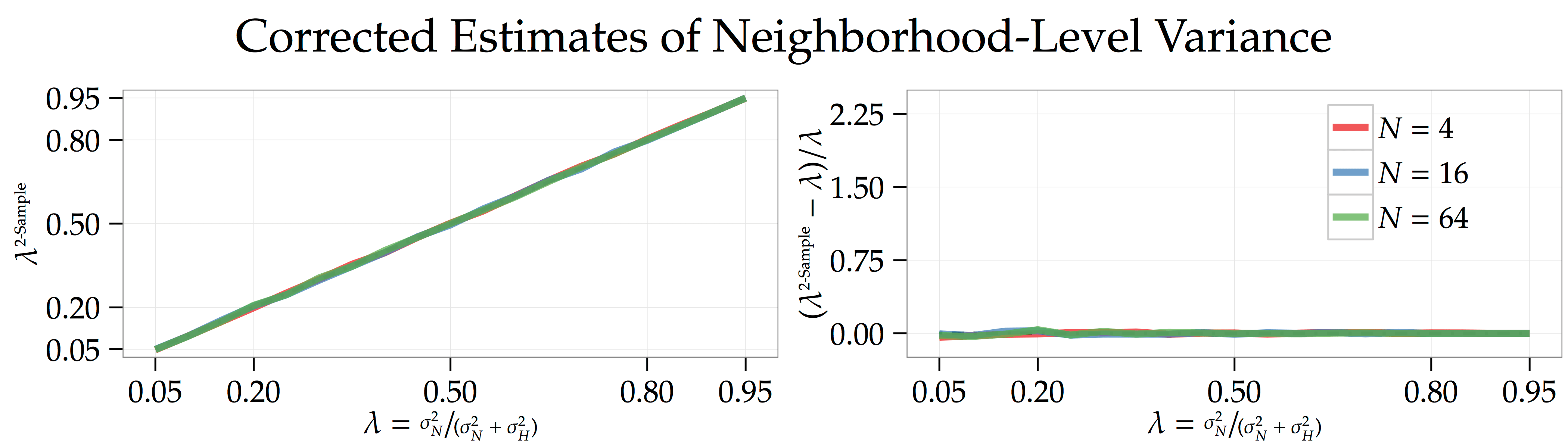
where and denote a collection of cleverly-chosen right-hand-side variables that I define below. The key insight is that, if you define these variables correctly, then you can read off both the neighborhood-level and house-level variation from the coefficients.

Here’s how. First, to create the variables that define the neighborhood-level variation, , randomly pair-off each neighborhood within the county so that there are neighborhood pairs. Then create the variables:

(8)  

So, the first of these variables, , compares the average price in the first neighborhood to the average price in the second neighborhood, meaning that the variable is mean zero. The scaling by then ensures that for all .

Next, to create the variables that define the house-level variation, , randomly pair-off each house within a neighborhood so that there are house pairs within each neighborhood and pairs in total. Then, use these house pairs to create the variables:

(9)  

So, the first of these variables, , compares the price of the first house to the price of the second house, meaning that the variable is mean zero. The scaling by ensures that for all

Because these right-hand-side variables are orthogonal to one another,

(10)  

we can then use their coefficients to estimate

(11)  

and thus generated an unbiased estimate of :

(12)  

The simulations below [code] use the exact sample parameter values as above but calculate using this correction. All of the earlier bias disappears.

1. Motivating Example

A Popular Goal. Financial economists have been looking for variables that predict stock returns for as long as there have been financial economists. For some recent examples, think about Jegadeesh and Titman (1993), which shows that a stock’s current returns are predicted by the stock’s returns over the previous months, Hou (2007), which shows that the current returns of smallest stocks in an industry are predicted by the lagged returns of the largest stocks in the industry, and Cohen and Frazzini (2008), which shows that a stock’s current returns are predicted by the lagged returns of its major customers.

Two-Step Process. When you think about it, finding these sorts of variables actually consists of two separate problems, identification and estimation. First, you have to use your intuition to identify a new predictor, , and then you have to use statistics to estimate this new predictor’s quality,

(1)  

where and are estimated coefficients, is the return on the th stock, and is the regression residual. If knowing reveals a lot of information about what a stock’s future returns will be, then and the associated will be large.

Can’t Always Use Intuition. But, modern financial markets are big, fast, and dense. Predictability doesn’t always occur at scales that are easy for people to intuit, making the standard approach to tackling the first problem problematic. For instance, the lagged returns of the Federal Signal Corporation were a significant predictor for more than of all NYSE-listed telecom stocks during a -minute stretch on October th, 2010. Can you really fish this particular variable out from the sea of spurious predictors using intuition alone? And, how exactly are you supposed to do this in under minutes?

Using Statistics Instead. In a recent working paper (link), Mao Ye, Adam Clark-Joseph, and I show how to replace this intuition step with statistics and use the least absolute shrinkage and selection operator (LASSO) to identify rare, short-lived, “sparse” signals in the cross-section of returns. This post uses simulations to show how the LASSO can be used to forecast returns.

2. Using the LASSO

LASSO Definition. The LASSO is a penalized-regression technique that was was introduced in Tibshirani (1996). It simultaneously identifies and estimates the most important coefficients using a far shorter sample period by betting on sparsity—that is, by assuming only a handful of variables actually matter at any point in time. Formally, using the LASSO means solving the problem below,

(2)  

where is a stock’s return at time , is a -dimensional vector of estimated coefficients, is the value of th predictor at time , is the number of time periods in the sample, and is a penalty parameter. Equation (2) looks complicated at first, but it’s not. It’s a simple extension of an OLS regression. In fact, if you ignore the right-most term—the penalty function, —then this optimization problem would simply be an OLS regression.

Penalty Function. But, it’s this penalty function that’s the secret to the LASSO’s success, allowing the estimator to give preferential treatment to the largest coefficients and completely ignore the smaller ones. To better understand how the LASSO does this, consider the solution to Equation (2) when the right-hand-side variables are uncorrelated and have unit variance:

(3)  

Here, represents what the standard OLS coefficient would have been if we had an infinite amount of data, , and . On one hand, this solution means that, if OLS would have estimated a large coefficient, , then the LASSO is going to deliver a similar estimate, . On the other hand, the solution implies that, if OLS would have estimated a sufficiently small coefficient, , then the LASSO is going to pick . Because the LASSO can set all but a handful of coefficients to zero, it can be used to identify the most important predictors even when the sample length is much shorter than the number of possible predictors, . Morally speaking, if only of the predictors are non-zero, then you should only need a few more than observations to select and then estimate the size of these few important coefficients.

3. Simulation Analysis

I run simulations to show how to use the LASSO to forecast future returns. You can find all of the relevant code here.

Data Simulation. Each simulation involves generating returns for stocks for periods. Each period, the returns of all stocks are governed by the returns of a subset of stocks, , together with an idiosyncratic shock,

(4)  

where . This cast of sparse signals changes over time, leading to the time subscript on . Specifically, I assume that there is a chance that each signal changes every period, so each signal lasts lasts periods on average.

Fitting Models to the Data. For each period from to , I estimate the LASSO on the first stock, , as defined in Equation (2) using the previous periods of data where the possible predictors are the stocks. This means using time periods to estimate a model with potential right-hand-side variables. As useful benchmarks, I also estimate the autoregressive model from Equation (1) and an oracle regression. In this specification, I estimate an OLS regression with the true predictors as the right-hand-side variables. Obviously, in the real-world you don’t know what the true predictors are, but this specification gives an estimate of the best fit you could achieve. After fitting each model to the previous periods of data, I then make an out-of-sample forecast in the st period.

Forecasting Regressions. I then check how closely these forecasts line up with the realized returns of the first asset by analyzing the adjusted statistics from a bunch of forecasting regressions. For example, I take the LASSO’s return forecast in periods to and estimate the regression below,

(5)  

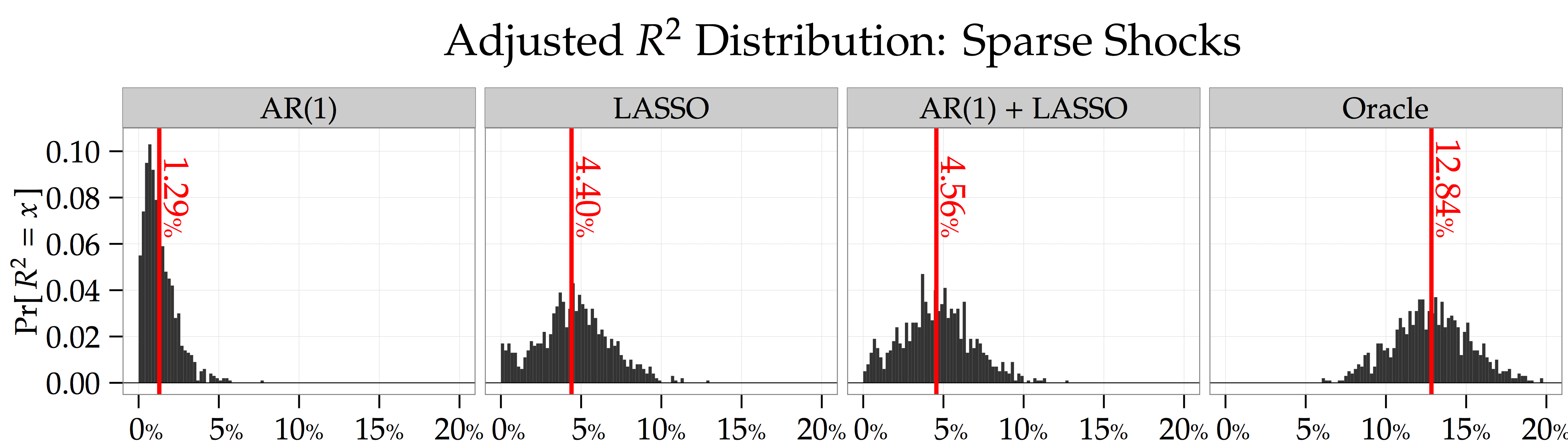
where and are estimated coefficients, denotes the first stock’s realized return in period , denotes the LASSO’s forecast of the first stock’s return in minute , and represent the mean and standard deviation of this out-of-sample forecast from period to , and is the regression residual. The figure below shows that the average adjusted- statistic from simulations is for the LASSO; whereas, this statistic is only when making your return forecasts using an autoregressive model,

(6)  

4. Tuning Parameter

Penalty Parameter Choice. Fitting the LASSO to the data involves selecting a penalty parameter, . I do this by selecting the penalty parameter that has the highest out-of-sample forecasting during the first periods of the data. This is why the forecasting regressions above only use data starting at instead of . The figure below shows the distribution of penalty parameter choices across the simulations. The discrete jumps come from the discrete grid of possible s that I considered when running the code.

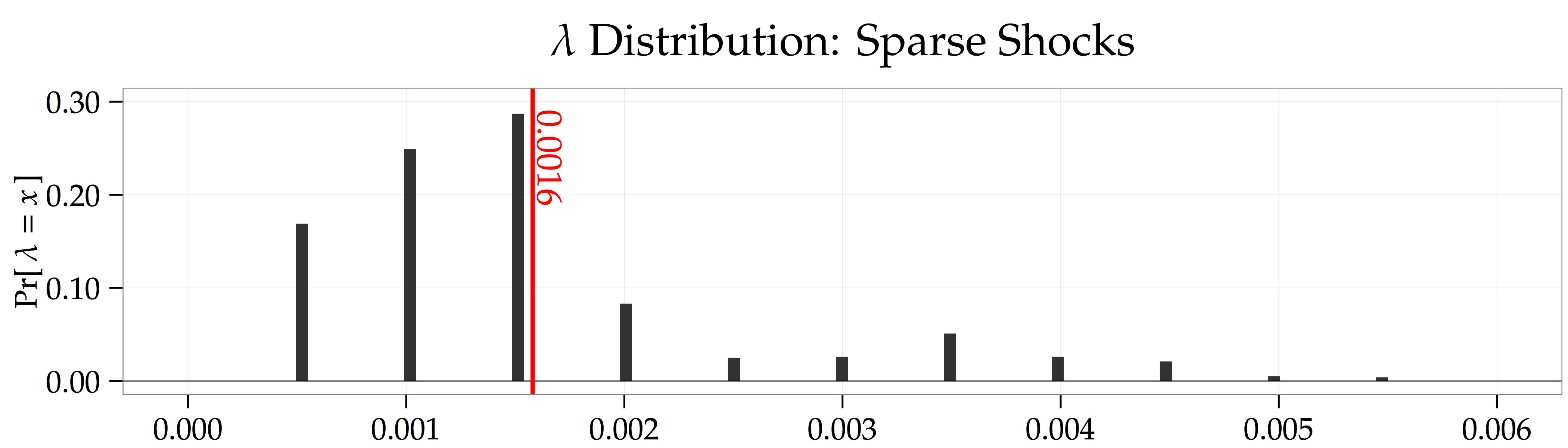
Number of Predictors. Finally, if you look at the panel labeled “Oracle” in the adjusted figure, you’ll notice that the LASSO’s out-of-sample forecasting power is about a third of the true model’s forecasting power, . This is because the LASSO doesn’t do a perfect job of picking out the sparse signals. The right panel of the figure below shows that the LASSO usually only picks out the most important of these signals. What’s more, the left panel shows that the LASSO also locks onto lots of spurious signals. This result suggests that you might be able to improve the LASSO’s forecasting power by choosing a higher penalty parameter, .

5. When Does It Fail?

Placebo Tests. I conclude this post by looking at two alternative simulations where the LASSO shouldn’t add any forecasting power. In the first alternative setting, there are no shocks. That is, the returns for the stocks are simulated using the model below,

(7)  

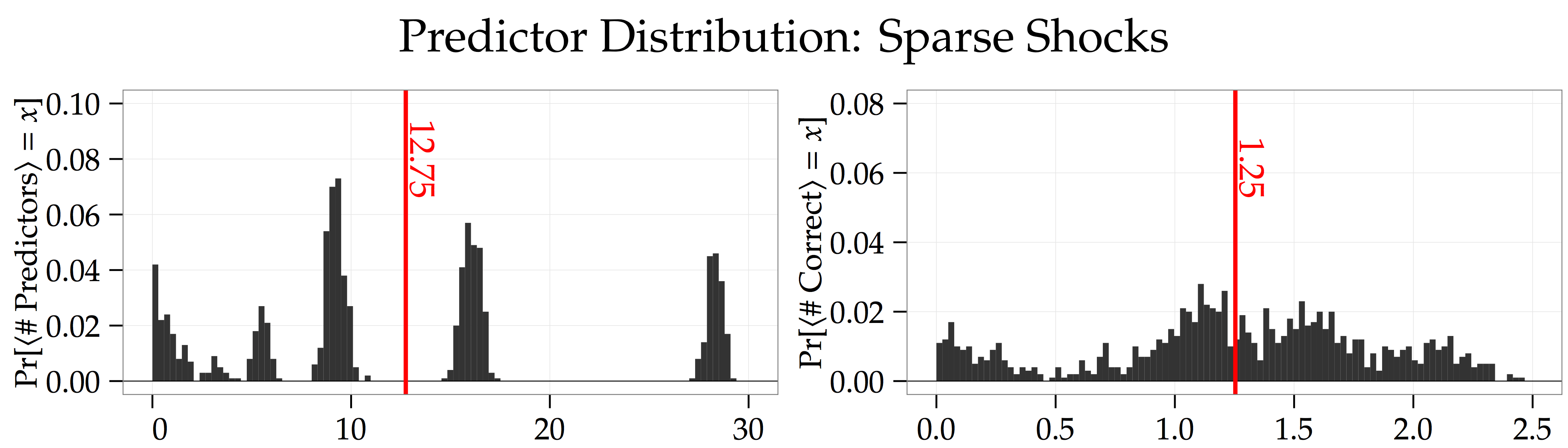
In the second setting, there are too many shocks: . The figures below show that, in both these settings, the LASSO doesn’t add any forecasting power. Thus, running these simulations offers a pair of nice placebo tests showing that the LASSO really is picking up sparse signals in the cross-section of returns.

1. Motivating Example

In several earlier posts (e.g., here and here) I’ve talked about the two well-known information-based asset-pricing models, Grossman and Stiglitz (1980) and Kyle (1985). But, there are lots of situations that don’t really fit with either of these two models. For one thing, uninformed speculators often recognize that they’re going to have a price impact, so it’s at odds with Grossman and Stiglitz (1980). For another thing, uninformed speculators typically use limit orders, so it’s at odds with Kyle (1985).

This post outlines the Kyle (1989) model which studies speculators that place limit orders and recognize their own price impact.

2. Market Structure

Assets. There is a single trading period and a single risky asset with a price of . This risky asset’s liquidation value is . For example, you might think about the asset as a stock that’ll have a value of after some important news announcement tomorrow. It’s just that, right now, you don’t know which direction the news will go.

Traders. There are kinds of traders: noise traders, informed speculators, and uninformed speculators. Noise traders demand shares of the risky asset. There are informed speculators and uninformed speculators. Both informed and uninformed traders have an initial endowment of (this is just a normalization) and exponential utility with risk-aversion parameter ,

(1)  

where denotes the number of shares demanded by a speculator.

Information. Prior to trading, each informed speculator gets a private signal and has a demand schedule . That is, he has in mind a function which tells him how many shares to demand at each possible price, , given his private signal, . Assume that the informed speculators’ signals can be written as

(2)  

where . Each uninformed speculator has a demand schedule .

3. Equilibrium Concept

Definition. An equilibrium is a set of demand schedules, for the informed speculators and for the uninformed speculators, and a price function such that (a) markets clear,

(3)  

and (b) both informed and uninformed speculators optimize,

(4)  

Both informed and uninformed speculators understand the relationship between prices and the random variables and . Prices will not be fully revealing due to the presence of noise-trader demand, .

Refinements. I make a pair of additional restrictions on the set of equilibria. Namely, I look only for linear, symmetric equilibria where the informed speculators’ demand schedules can be written as

(5)  

the uninformed-speculators’ demand schedules can be written as

(6)  

and the price can be written as

(7)  

4. Information Updating

Price Impact. If we substitute the linear demand schedules for the informed and uninformed speculators into the market-clearing condition, then we get a formula for the price,

(8)  

Thus, if noise traders supply one additional share, then the price drops by . Next, I define the same object for informed and uninformed speculators. That is, taking the demand schedules of the other speculators as given, how much will the price change if the th informed speculator or th uninformed speculator increases his demand by share? This question defines the residual supply curves,

(9)  

Imperfect competition is present because each trader recognizes that if he submits a different schedule, the resulting equilibrium price may change.

Forecast Precision. Informed speculator’s forecast precision is given via Bayesian updating as:

(10)  

represents the fraction of the precision from the other informed speculators revealed to the th informed speculator by the price. The corresponding forecast precision for uninformed speculator is:

(11)  

represents the fraction of the precision of the informed speculators revealed to the th uninformed speculator by the price. Clearly, prices become perfectly revealing as .

Posterior Beliefs. The th informed speculator’s posterior beliefs about the risky asset’s liquidation value is a weighted average of the public price signal and his private signal,

(12)  

Uninformed speculators form their posterior beliefs solely on the public price signal,

(13)  

5. Optimal Demand

Informed Demand. The th informed speculator observes his private signal, , and the price implied by the demand of the other traders, . He then solves the optimization problem below,

(14)  

But, the residual demand curve, , is related to the actual price, . So, after a little bit of rearranging, we can write the informed speculators’ optimal demand schedules as

(15)  

Uninformed Demand. The th uninformed speculator observes only the price implied by the demand of the other traders, . He then solves the optimization problem below,

(16)  

Using the exact same tricks, we can write the uninformed speculators’ optimal demand schedule as

(17)  

6. Endogenous Parameters

Next, it’s useful to define a couple of additional parameters.

Information Incidence. First, define the information incidence as

(18)  

This new parameter represents the increase in the equilibrium price when the th informed speculator’s valuation of the risky asset goes up by as a result of a higher signal realization, . For trader ‘s valuation to rise by , his private signal must rise by a factor of , and prices move by a factor of for every increase in the th informed speculator’s private signal, . In equilibrium, it turns out that .

Marginal Market Share. Next, define two parameters capturing the marginal market share of the informed and uninformed speculators,

(19)  

Here’s how you interpret : if noise traders demand additional share, then the quantity traded by each informed speculator increases by shares. Likewise, captures the amount of additional trading that each uninformed speculator does in response to a share increase in noise-trader demand.

7. Model Solution

Kyle (1989) shows that there exists a unique symmetric linear equilibrium if , , , and . This equilibrium is characterized by a system of equations and unknowns, , subject to the constraints that , , , and .

Equation 1. The first equation is the easiest. If noise traders demand an additional share, then someone has to sell it to them. Informed speculators tend to adjust their demand by shares, and uninformed speculators tend to adjust their demand by shares. Thus, because there are informed speculators and uninformed speculators, we have the market-clearing condition below:

(20)  

Equation 2. Next, we turn to the second equation, which characterizes the informed speculator’s demand response to price changes, , via the endogenous parameter ,

(21)  

This equation links how unresponsive prices are to a increase in an informed speculator’s private signal, , to the product of how uninformative prices are about other informed speculators’ signals, , and how little each informed speculator has to trade in response to a share increase in noise-trader demand, . After all, if informed speculators don’t have to trade that often—i.e., —and prices don’t really reveal much of their private signal to other informed speculators when they do—i.e., , then prices shouldn’t be moving that much in response to private shocks—i.e., .

Equation 3. The third equation is much more directly an equilibrium characterization of ,

(22)  

Informed speculators are going to trade more aggressively in response to a increase in their private signal when their private signal is more precise (i.e., is big), when they are closer to risk neutral (i.e., is small), when prices don’t reveal much about their private signal to other informed speculators (i.e., because ), or when prices don’t move much when informed speculators trade on their private information (i.e., because ). Notice that this last effect is second order when is small.

Equation 4. Finally, let’s have a look at equation, which characterizes the uninformed speculator’s demand response to price changes, , via the endogenous parameter ,

(23)  

I don’t have any clean way to analyze the right-hand side of this equation, but it is possible to show that the right-hand side will only be if —that is, if there are lots of small uninformed speculators. What’s more, we know from Equation (13) that prices will only be an unbiased estimate of the uninformed speculators’ beliefs if:

(24)  

If we rearrange the left-hand side of the equation a bit,

(25)  

we see that prices can only be unbiased if there are lots of small uninformed speculators, just like in Grossman and Stiglitz (1980). Otherwise, prices overreact—that is, .

8. Numerical Analysis

To make sure that I’ve understood how to solve the model correctly, I solved for the equilibrium parameters numerically when , , , , and as the precision of noise-trader demand volatility ranges from to . You can find the code here. I’ve plotted some of the results below.

1. Motivating Example

Jegadeesh and Titman (1993) show that, if you rank stocks according to their returns over the previous months, then the past winners will outperform the past losers by per month over the next months. But, the authors don’t just test this particular strategy. They also test strategies that rank stocks over the previous , , and months and strategies which hold stocks for the next , , and months, too. Clearly, if they test enough hypotheses, then some of these tests are going to appear statistically significant by pure chance. To address this concern in the original paper, the authors use the Bonferroni method.

This post shows how to use an alternative method—namely, controlling the false-discovery rate—to identify statistically significant results when testing multiple hypotheses.

2. Bonferroni Method

First, here’s the logic behind the Bonferroni method. Suppose you want to run different hypothesis tests, . Let if the th null hypothesis is true and if the th null hypothesis is false (i.e., should be rejected). Let denote the p-value associated with some test statistic for the th hypothesis. If there were just one test, then we should simply reject the null whenever . But, if there are many tests, then this no longer works. If you look at a lot of hypotheses, then of the p-values should be less than even if for all of them. The Bonferroni method suggests correcting this problem by lowering the p-value associated with the significance level and only rejecting the null hypothesis when

(1)  

i.e., if there are hypothesis tests, then only reject the null at the significance level when the p-value is less than rather than .

This is a nice start, but it turns out that the Bonferroni method is way too strict. Imagine drawing samples of observations from different normal distributions. All samples have the same standard deviation, , but not all of the sample have the same mean. have a mean of , and the rest have a mean of . The figure below shows that, if we use the Bonferroni method to identify which of the samples have a non-zero mean, then we’re only going to choose samples. But, by construction, we know that samples had a non-zero mean! We should be rejecting the null -times more often!

3. False-Discovery Rate

Now, let’s talk about false-discovery rates. Define as the total number hypotheses that you reject at the significance level. Similarly, define as the number of hypotheses that you reject at the significance level where the null was actually true—i.e., these are false rejections. The false-discovery rate is then

(2)  

Let’s return to the numerical example above to clarify this definition. Suppose we had a test that identified all cases where the sample mean was , . If we wanted a false-discovery rate , then this test could produce at most false rejections, . If the test identified only half of the cases where the sample mean was , , then this test could produce at most one false rejection, .

Benjamini and Hochberg (1995) first introduced the idea that you could use the false-discovery rate to adjust statistical-significance tests when exploring multiple hypotheses. Here’s their recipe. First, run all of your tests and order the resulting p-values,

(3)  

Then, for a given false-discovery rate, , define as

(4)  

Benjamini and Hochberg (1995) showed that, if you reject any null hypothesis where

(5)  

then , guaranteed. If we apply the false-discovery-rate procedure to the same numerical example from above using the threshold, then we see that as the number of hypotheses gets large, , the fraction of rejected null hypotheses hovers around . Improvement! It’s no longer shrinking to . Notice that neither method allows us to pick out the full of null hypotheses that should be rejected in the simulation.

4. Why’s This So?

It’s pretty clear how the Bonferroni method works. If there are lots of hypotheses and you are worried about rejecting the null by pure chance, then just make it harder to reject the null. i.e., lower the threshold for significant p-values. It’s much less clear, though, how the false-discovery-rate screening process works. All you get is a recipe and a guarantee. If you do the list of things prescribed by Benjamini and Hochberg (1995), then you’ll falsely reject no more than of your null hypotheses. Let’s explore the proof of this result from Storey, Taylor and Siegmund (2003) to better understand where this guarantee comes from.

What does it mean to have a useful test? Well, if (null is true), then is drawn randomly from a uniform distribution, . However, if you have a useful test statistic, then if (null is false), then is drawn from some other distribution, that is more concentrated around . The distribution of p-values is then given by

(6)  

If we reject all p-value less than , then with a little bit of algebra we can see that

(7)  

where the last step uses the fact that and denotes “big-O” notation. Since p-values are drawn from a uniform distribution when the null hypothesis is true, we know that . Thus, we can simplify even further:

(8)  

Now comes the trick. can be anything we want between and . So, let’s choose as one of the ordered p-values, . If we do this, then and

(9)  

If we set the right-hand side equal to the false-discovery-rate tolerance, , and solve for , then we get the threshold value for in Benjamini and Hochberg (1995),

(10)  

If we only reject hypotheses where , then our false-discovery rate is capped at .