Alex – Page 7 – Research Notebook

The Characteristic Scale of House-Price Variation

January 24, 2016 by Alex

1. Introduction

There are many reasons why two houses might have different prices. To start with, one house might just be larger or have a better layout than the other. Let’s call these sorts of house-to-house differences “fine-grained”. But, prices can also vary for reasons that have nothing to do with the houses themselves. Even if two houses are physically identical, one house might sit in a more attractive neighborhood or belong to a better school district. Let’s call such differences over larger scales “coarse-grained”.

Different scales dominate in different places. In some counties, most of the price variation comes from fine-grained, house-to-house differences. Think about Los Angeles, CA where there is a lot of heterogeneity in the age and quality of the housing stock, even for houses that are right next door to one another. But, there are also coarse-grained counties where most of the house-price variation occurs over much larger scales. Think about Orange County, CA where the typical house is part of a subdivision. While there are lots of differences between subdivisions in Orange County, all the houses within each subdivision are typically built in a similar style by a single company at the exact same time.

This post shows how to estimate the characteristic scale of house-price variation in a county. That is, it shows how to tell if a county is fine-grained like Los Angeles, coarse-grained like Orange County, or somewhere in between. To do this, I introduce a new scale-specific variance estimator based on the Allan variance. This estimator decomposes the cross-sectional house-price variation in a given county into scale-specific components such as the amount of variation that arises from comparing randomly selected houses or the amount of variation that arises from comparing randomly selected neighborhoods.

Why not just compare the variance of the individual house prices to the variance of the neighborhood-level averages? The answer is simple: those calculations aren’t independent. Fine-grained counties with lots of house-to-house variation will mechanically have more variance in their average neighborhood-level prices. Just imagine the extreme case where all of the variation comes from house-to-house differences and each house’s price is independently drawn from the same normal distribution, $p_h \overset{\scriptscriptstyle \mathrm{iid}}{\sim} \mathsf{N}(\bar{p}, \, \sigma_H^2)$ . In a world where the $n$ th neighborhood has $L$ houses, the variance of the neighborhood-level average price, $\mathsf{E}(p_h|h \in n) = \hat{\mu}_n$ , would be increasing in the amount of house-to-house variation, $\mathsf{Var}(\hat{\mu}_n)=\sfrac{\sigma_H^2}{L}$ . I use this new scale-specific estimator because I don’t want to confuse these sorts of emergent neighborhood-level fluctuations with the honest-to-goodness neighborhood-level differences.

2. Data-Generating Process

Consider a county with $H$ houses and $N$ neighborhoods where there are $L \geq 2$ houses in each neighborhood so that $(L \cdot N) = H$ . Suppose that house prices are the sum of a neighborhood-level value and a house-level value,

(1) $\begin{align*} p_h &= {\textstyle \sum_n} \mu_n \cdot 1_{\{ h \in n \}} + \theta_h, \end{align*}$

with $\mu_n \overset{\scriptscriptstyle \mathrm{iid}}{\sim} \mathsf{N}(0, \, \sigma_N^2)$ and $\theta_h \overset{\scriptscriptstyle \mathrm{iid}}{\sim} \mathsf{N}(0, \, \sigma_H^2)$ . Think about neighborhood-level values as the quality of the local school district or the attractiveness of the nearby restaurant scene. This value is coarse-grained. You can have a mansion or a hovel in a nice school district. The house-level value, by contrast, relates to the characteristics of each particular house. This value is fine-grained.

Given this data-generating process, we know that a fraction

(2) $\begin{align*} \lambda = {\textstyle \frac{\sigma_N^2}{\sigma_N^2 + \sigma_H^2}} \end{align*}$

of the variation in house prices comes from neighborhood-level differences. This is the object of interest in the current post. If $\lambda$ is close to $1$ , then the county is dominated by coarse-grained variation in house prices and looks like Orange County, CA. If $\lambda$ is close to $0$ , then the county is dominated by fine-grained variation in house prices and looks more like Los Angeles, CA. In the analysis below, I’m going to show how to estimate $\lambda$ in simulated data.

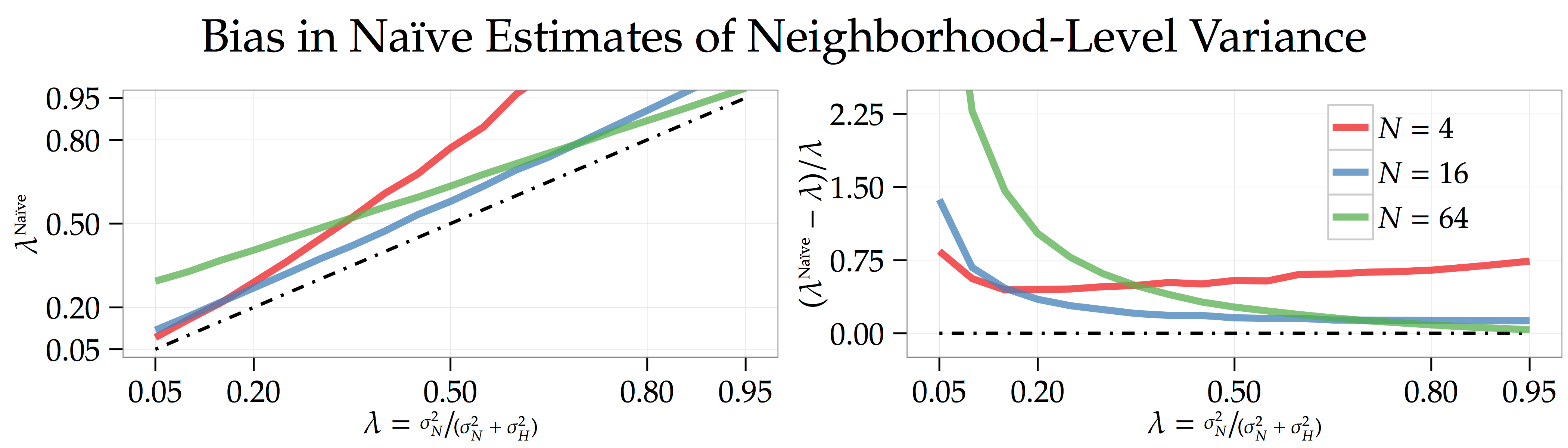
3. Naïve Estimate of λ

One way to estimate $\lambda$ would be to look at a variance ratio. You might first compute the average price in each neighborhood,

(3) $\begin{align*} \hat{\mu}_n = \mathsf{E}(p_h|h \in n) = {\textstyle \frac{1}{L} \cdot \sum_{h \in n}} p_h, \end{align*}$

and then look at the ratio of the variance of the neighborhood-level average prices to the total house-price variance:

(4) $\begin{align*} \lambda^{\scriptscriptstyle\text{Na\"{i}ve}} = {\textstyle \frac{ \mathsf{Var}(\hat{\mu}_n) }{ \mathsf{Var}(p_h) } }. \end{align*}$

The thought process behind this calculation is really simple. If different neighborhoods have very different prices, then there should be a lot of variation in the average neighborhood-level price. In fact, it turns out to be too simple. While it is true that this naïve calculation will generate a higher $\lambda$ in counties with lots of coarse-grained neighborhood-level variation, it will also be high in counties with lots of fine-grained house-to-house variation.

To see why, let’s look at the variance of the average price in each county:

(5) $\begin{align*} \mathsf{Var}(\hat{\mu}_n) &= {\textstyle \frac{1}{N} \cdot \sum_n} (\hat{\mu}_n - \hat{\mu} )^2 \\ &= \underbrace{{\textstyle \frac{1}{N} \cdot \sum_n} (\mu_n - 0)^2}_{\sigma_N^2} + \underbrace{{\textstyle \frac{1}{N} \cdot \sum_n} (\hat{\mu}_n - \mu_n)^2}_{\sfrac{\sigma_H^2}{L}} - \underbrace{{\textstyle \frac{1}{N} \cdot \sum_n}(\hat{\mu} - 0)^2}_{\sfrac{\sigma_N^2}{N} + \sfrac{\sigma_H^2}{H}}. \end{align*}$

This variance consists of $3$ parts: the true neighborhood-level variance, $\sigma_N^2$ ; differences in neighborhood-level prices from fine-grained variation, $\sfrac{\sigma_H^2}{L}$ ; and, a correction for the unknown sample mean, $-\left( \sfrac{\sigma_N^2}{N} + \sfrac{\sigma_H^2}{H}\right)$ . If we solve for the true amount of neighborhood-level variation,

(6) $\begin{align*} \sigma_N^2 &= {\textstyle \frac{N}{N - 1}} \cdot \left( \, \mathsf{Var}(\hat{\mu}_n) - {\textstyle \frac{N - 1}{H}} \cdot \sigma_H^2 \, \right), \end{align*}$

we see that it’s going to be smaller than the variation in neighborhood-level average prices. Counties with lots of fine-grained, house-to-house differences look like they have too much neighborhood-level house-price variation. What’s more, in the simulations plotted below [code] where the county has $H = 256$ houses, you can see that the nature of this bias is going to vary in a non-trivial way as the number of neighborhoods and the amount of coarse-grained, neighborhood-level variation changes.

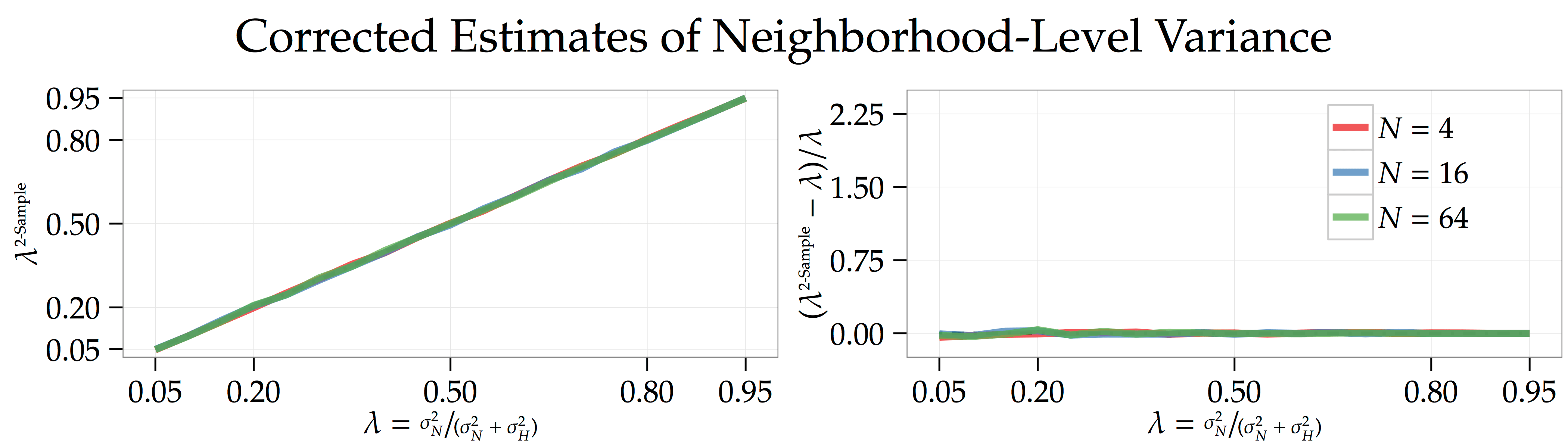
4. Corrected Estimate of λ

In order to fix the problem, we need a way of simultaneously estimating neighborhood-level and house-level price variation and then using the second estimate to correct the bias in the first. It turns out that you can do this by running a simple cross-sectional regression,

(7) $\begin{align*} p_h &= \hat{\alpha} + {\textstyle \sum_n} \left\{ \, {\textstyle \sum_{j = 1}^{N/2}} \hat{\beta}_j \cdot x_j(n) \, \right\} \cdot 1_{\{ h \in n \}} + {\textstyle \sum_{k=1}^{H/2}} \hat{\gamma}_k \cdot y_k(h) + \epsilon_h, \end{align*}$

where $\{ x_j(n) \}_{j=1}^{N/2}$ and $\{ y_k(h) \}_{k=1}^{H/2}$ denote a collection of cleverly-chosen right-hand-side variables that I define below. The key insight is that, if you define these variables correctly, then you can read off both the neighborhood-level and house-level variation from the coefficients.

Here’s how. First, to create the variables that define the neighborhood-level variation, $\{ x_j(n) \}_{j=1}^{N/2}$ , randomly pair-off each neighborhood within the county so that there are $\sfrac{N}{2}$ neighborhood pairs. Then create the variables:

(8) $\begin{align*} \mathbf{x}_1 &= {\textstyle \sqrt{\frac{1}{2} \cdot \left(\frac{H - 1}{2 \cdot (\sfrac{H}{N})}\right)}} \times \left[ \begin{array}{ccc:ccc:ccc:ccc:c} 1 & \cdots & \phantom{-}1 & -1 & \cdots & -1 & 0 & \cdots & \phantom{-}0 & \phantom{-}0 & \cdots & \phantom{-}0 & \cdots \end{array} \right]^{\top} \\ \mathbf{x}_2 &= {\textstyle \sqrt{\frac{1}{2} \cdot \left(\frac{H - 1}{2 \cdot (\sfrac{H}{N})}\right)}} \times \left[ \begin{array}{ccc:ccc:ccc:ccc:c} 0 & \cdots & \phantom{-}0 & \phantom{-}0 & \cdots & \phantom{-}0 & 1 & \cdots & \phantom{-}1 & -1 & \cdots & -1 & \cdots \end{array} \right]^{\top} \\ &\vdots \end{align*}$

So, the first of these variables, $\mathbf{x}_1$ , compares the average price in the first neighborhood to the average price in the second neighborhood, meaning that the variable is mean zero. The scaling by $\sqrt{\frac{1}{2} \cdot \left(\frac{H - 1}{2 \cdot (\sfrac{H}{N})}\right)}$ then ensures that $\sfrac{1}{2} = \mathsf{Var}(\mathbf{x}_j)$ for all $j = 1, 2, \ldots, \sfrac{N}{2}$ .

Next, to create the variables that define the house-level variation, $\{ y_k(h) \}_{k=1}^{H/2}$ , randomly pair-off each house within a neighborhood so that there are $\sfrac{L}{2}$ house pairs within each neighborhood and $\sfrac{H}{2}$ pairs in total. Then, use these house pairs to create the variables:

(9) $\begin{align*} \mathbf{y}_1 &= {\textstyle \sqrt{\frac{1}{2} \cdot \left( \frac{H-1}{2 \cdot 1} \right)}} \times \left[ \begin{array}{ccccccc:c} 1 & -1 & 0 & \phantom{-}0 & \cdots & 0 & \phantom{-}0 & \cdots \end{array} \right]^{\top} \\ \mathbf{y}_2 &= {\textstyle \sqrt{\frac{1}{2} \cdot \left(\frac{H-1}{2 \cdot 1}\right)}} \times \left[ \begin{array}{ccccccc:c} 0 & \phantom{-}0 & 1 & -1 & \cdots & 0 & \phantom{-}0 & \cdots \end{array} \right]^{\top} \\ &\vdots \end{align*}$

So, the first of these variables, $\mathbf{y}_1$ , compares the price of the first house to the price of the second house, meaning that the variable is mean zero. The scaling by $\sqrt{\frac{1}{2} \cdot \left(\frac{H - 1}{2 \cdot 1}\right)}$ ensures that $\sfrac{1}{2} = \mathsf{Var}(\mathbf{y}_k)$ for all $k = 1, 2, \ldots, \sfrac{H}{2}$

Because these right-hand-side variables are orthogonal to one another,

(10) $\begin{align*} 0 = \mathsf{Cov}(\mathbf{x}_j, \mathbf{x}_{j'}) = \mathsf{Cov}(\mathbf{y}_k, \mathbf{y}_{k'}) = \mathsf{Cov}(\mathbf{x}_j, \mathbf{y}_{k}), \end{align*}$

we can then use their coefficients to estimate

(11) $\begin{align*} \tilde{\sigma}_H^2 &= {\textstyle \sum_{k=1}^{H/2}}\hat{\gamma}_k^2 \\ \text{and} \quad \tilde{\sigma}_N^2 &= {\textstyle \sum_{j=1}^{N/2}} \hat{\beta}_j^2 - {\textstyle \frac{\tilde{\sigma}_H^2}{\sfrac{H}{N}}}, \end{align*}$

and thus generated an unbiased estimate of $\lambda$ :

(12) $\begin{align*} \lambda^{\scriptscriptstyle \text{2-Sample}} &= {\textstyle \frac{\tilde{\sigma}_N^2}{\tilde{\sigma}_N^2 + \tilde{\sigma}_H^2}}. \end{align*}$

The simulations below [code] use the exact sample parameter values as above but calculate $\lambda$ using this correction. All of the earlier bias disappears.

Using the LASSO to Forecast Returns

December 5, 2015 by Alex

1. Motivating Example

A Popular Goal. Financial economists have been looking for variables that predict stock returns for as long as there have been financial economists. For some recent examples, think about Jegadeesh and Titman (1993), which shows that a stock’s current returns are predicted by the stock’s returns over the previous $12$ months, Hou (2007), which shows that the current returns of smallest stocks in an industry are predicted by the lagged returns of the largest stocks in the industry, and Cohen and Frazzini (2008), which shows that a stock’s current returns are predicted by the lagged returns of its major customers.

Two-Step Process. When you think about it, finding these sorts of variables actually consists of two separate problems, identification and estimation. First, you have to use your intuition to identify a new predictor, $x_t$ , and then you have to use statistics to estimate this new predictor’s quality,

(1) $\begin{align*} r_{n,t} &= \hat{\theta}_0 + \hat{\theta}_1 \cdot x_{t-1} + \epsilon_{n,t}, \end{align*}$

where $\hat{\theta}_0$ and $\hat{\theta}_1$ are estimated coefficients, $r_{n,t}$ is the return on the $n$ th stock, and $\epsilon_{n,t}$ is the regression residual. If knowing $x_{t-1}$ reveals a lot of information about what a stock’s future returns will be, then $|\hat{\theta}_1|$ and the associated $R^2$ will be large.

Can’t Always Use Intuition. But, modern financial markets are big, fast, and dense. Predictability doesn’t always occur at scales that are easy for people to intuit, making the standard approach to tackling the first problem problematic. For instance, the lagged returns of the Federal Signal Corporation were a significant predictor for more than $70{\scriptstyle \%}$ of all NYSE-listed telecom stocks during a $34$ -minute stretch on October $5$ th, 2010. Can you really fish this particular variable out from the sea of spurious predictors using intuition alone? And, how exactly are you supposed to do this in under $34$ minutes?

Using Statistics Instead. In a recent working paper (link), Mao Ye, Adam Clark-Joseph, and I show how to replace this intuition step with statistics and use the least absolute shrinkage and selection operator (LASSO) to identify rare, short-lived, “sparse” signals in the cross-section of returns. This post uses simulations to show how the LASSO can be used to forecast returns.

2. Using the LASSO

LASSO Definition. The LASSO is a penalized-regression technique that was was introduced in Tibshirani (1996). It simultaneously identifies and estimates the most important coefficients using a far shorter sample period by betting on sparsity—that is, by assuming only a handful of variables actually matter at any point in time. Formally, using the LASSO means solving the problem below,

(2) $\begin{align*} \hat{\boldsymbol \vartheta} &= \underset{{\boldsymbol \vartheta} \in \mathbf{R}^Q}{\mathrm{arg}\,\mathrm{min}} \, \left\{ \, \frac{1}{2 \cdot T} \cdot \sum_{t=1}^T \left(r_t - \vartheta_0 - {\textstyle \sum_{q=1}^Q} \vartheta_q \cdot x_{q,t-1}\right)^2 + \lambda \cdot \sum_{q=1}^Q \left|\vartheta_q\right| \, \right\}, \end{align*}$

where $r_t$ is a stock’s return at time $t$ , $\hat{\boldsymbol \vartheta}$ is a $(Q \times 1)$ -dimensional vector of estimated coefficients, $x_{q,t-1}$ is the value of $q$ th predictor at time $(t-1)$ , $T$ is the number of time periods in the sample, and $\lambda$ is a penalty parameter. Equation (2) looks complicated at first, but it’s not. It’s a simple extension of an OLS regression. In fact, if you ignore the right-most term—the penalty function, $\lambda \cdot \sum_q \left|\vartheta_q\right|$ —then this optimization problem would simply be an OLS regression.

Penalty Function. But, it’s this penalty function that’s the secret to the LASSO’s success, allowing the estimator to give preferential treatment to the largest coefficients and completely ignore the smaller ones. To better understand how the LASSO does this, consider the solution to Equation (2) when the right-hand-side variables are uncorrelated and have unit variance:

(3) $\begin{align*} \hat{\vartheta}_q &= \mathrm{sgn}[\hat{\theta}_q] \cdot (|\hat{\theta}_q| - \lambda)_+. \end{align*}$

Here, $\hat{\theta}_q$ represents what the standard OLS coefficient would have been if we had an infinite amount of data, $\mathrm{sgn}[x] = \sfrac{x}{|x|}$ , and $(x)_+ = \max\{0,\,x\}$ . On one hand, this solution means that, if OLS would have estimated a large coefficient, $|\hat{\theta}_q| \gg \lambda$ , then the LASSO is going to deliver a similar estimate, $\hat{\vartheta}_q \approx \hat{\theta}_q$ . On the other hand, the solution implies that, if OLS would have estimated a sufficiently small coefficient, $|\hat{\theta}_q| < \lambda$ , then the LASSO is going to pick $\hat{\vartheta}_q = 0$ . Because the LASSO can set all but a handful of coefficients to zero, it can be used to identify the most important predictors even when the sample length is much shorter than the number of possible predictors, $T \ll Q$ . Morally speaking, if only $K \ll Q$ of the predictors are non-zero, then you should only need a few more than $K$ observations to select and then estimate the size of these few important coefficients.

3. Simulation Analysis

I run $1,000$ simulations to show how to use the LASSO to forecast future returns. You can find all of the relevant code here.

Data Simulation. Each simulation involves generating returns for $Q = 100$ stocks for $T = 1,150$ periods. Each period, the returns of all $Q=100$ stocks are governed by the returns of a subset of $K=5$ stocks, $\mathcal{K}_t$ , together with an idiosyncratic shock,

(4) $\begin{align*} r_{q,t} &= 0.15 \cdot \sum_{q' \in \mathcal{K}_t} r_{q',t-1} + 0.001 \cdot \epsilon_{q,t}, \end{align*}$

where $\epsilon_{q,t} \overset{\scriptscriptstyle \mathrm{iid}}{\sim} \mathrm{N}(0,1)$ . This cast of $K = 5$ sparse signals changes over time, leading to the time subscript on $\mathcal{K}_t$ . Specifically, I assume that there is a $1{\scriptstyle \%}$ chance that each signal changes every period, so each signal lasts lasts $\sfrac{(1 - 0.01)}{0.01} = 99$ periods on average.

Fitting Models to the Data. For each period from $t=151$ to $t=1,150$ , I estimate the LASSO on the first stock, $q=1$ , as defined in Equation (2) using the previous $T=50$ periods of data where the $Q$ possible predictors are the $Q=100$ stocks. This means using $T=50$ time periods to estimate a model with $Q=100$ potential right-hand-side variables. As useful benchmarks, I also estimate the autoregressive model from Equation (1) and an oracle regression. In this specification, I estimate an OLS regression with the $K=5$ true predictors as the right-hand-side variables. Obviously, in the real-world you don’t know what the true predictors are, but this specification gives an estimate of the best fit you could achieve. After fitting each model to the previous $50$ periods of data, I then make an out-of-sample forecast in the $51$ st period.

Forecasting Regressions. I then check how closely these forecasts line up with the realized returns of the first asset by analyzing the adjusted $R^2$ statistics from a bunch of forecasting regressions. For example, I take the LASSO’s return forecast in periods $t=151$ to $t=1,150$ and estimate the regression below,

(5) $\begin{align*} r_{1,t+1} &= \alpha + \beta \times \left( \frac{f_{1,t}^{\scriptscriptstyle \mathrm{LASSO}} - \mu^{\scriptscriptstyle \mathrm{LASSO}}}{\sigma^{\scriptscriptstyle \mathrm{LASSO}}} \right) + \varepsilon_{1,t+1}, \end{align*}$

where $\alpha$ and $\beta$ are estimated coefficients, $r_{1,t+1}$ denotes the first stock’s realized return in period $(t+1)$ , $f_{1,t}^{\scriptscriptstyle \mathrm{LASSO}}$ denotes the LASSO’s forecast of the first stock’s return in minute $(t+1)$ , $\mu^{\scriptscriptstyle \mathrm{LASSO}}$ and $\sigma^{\scriptscriptstyle \mathrm{LASSO}}$ represent the mean and standard deviation of this out-of-sample forecast from period $t=151$ to $t=1,150$ , and $\varepsilon_{1,t+1}$ 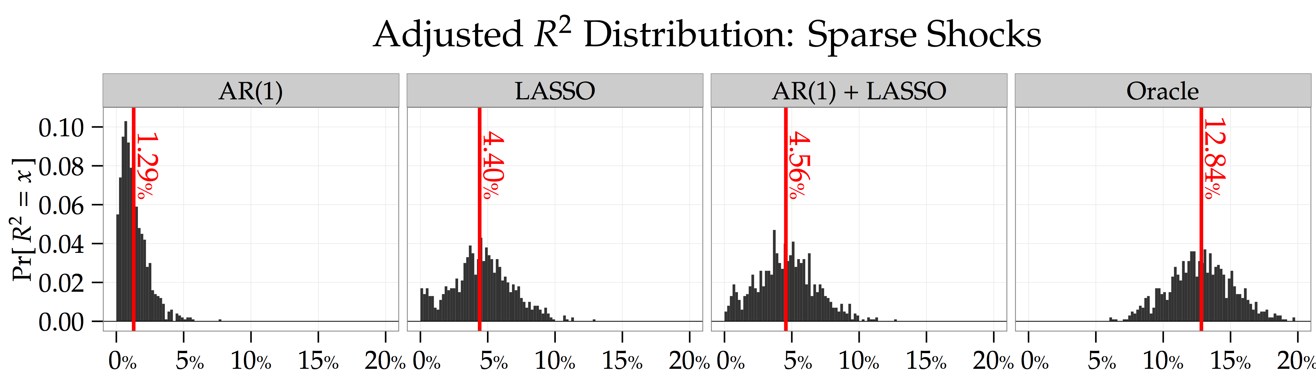is the regression residual. The figure below shows that the average adjusted- $R^2$ statistic from $1,000$ simulations is $4.40{\scriptstyle \%}$ for the LASSO; whereas, this statistic is only $1.29{\scriptstyle \%}$ when making your return forecasts using an autoregressive model,

(6) $\begin{align*} r_{1,t+1} &= \alpha + \beta \times \left( \frac{f_{1,t}^{\scriptscriptstyle \mathrm{OLS}} - \mu^{\scriptscriptstyle \mathrm{OLS}}}{\sigma^{\scriptscriptstyle \mathrm{OLS}}} \right) + \varepsilon_{1,t+1}. \end{align*}$

4. Tuning Parameter

Penalty Parameter Choice. Fitting the LASSO to the data involves selecting a penalty parameter, $\lambda$ . I do this by selecting the penalty parameter that has the highest out-of-sample forecasting $R^2$ during the first $100$ periods of the data. This is why the forecasting regressions above only use data starting at $t=151$ instead of $t=51$ . The figure below shows the distribution of penalty parameter choices across the $1,000$ simulations. 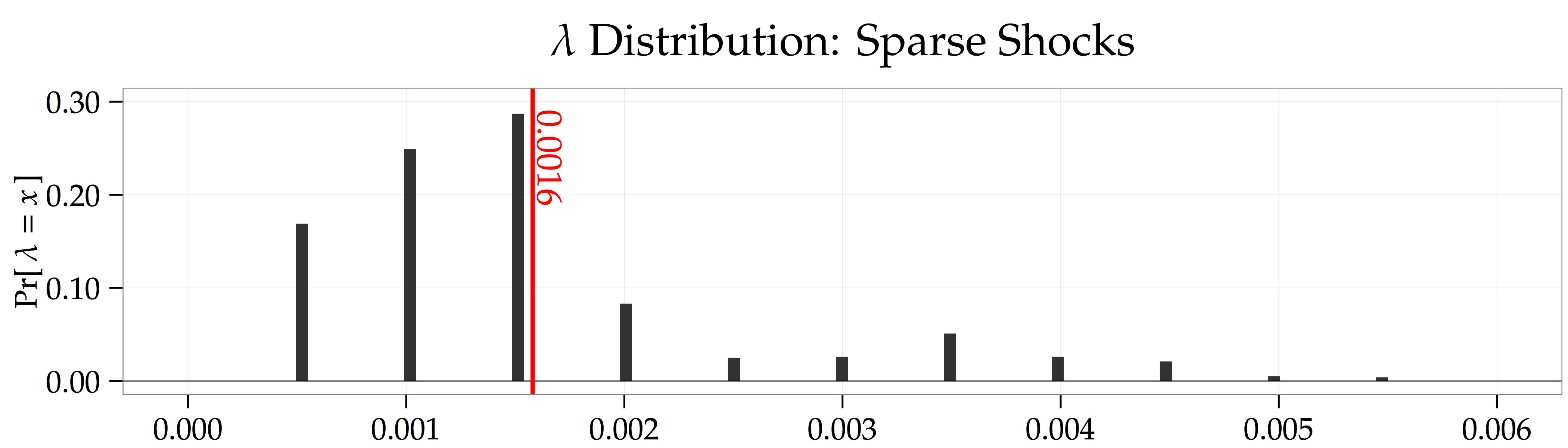The discrete $0.0005$ jumps come from the discrete grid of possible $\lambda$ s that I considered when running the code.

Number of Predictors. Finally, if you look at the panel labeled “Oracle” in the adjusted $R^2$ figure, you’ll notice that the LASSO’s out-of-sample forecasting power is about a third of the true model’s forecasting power, $\sfrac{4.40}{12.84} = 0.34$ . This is because the LASSO doesn’t do a perfect job of picking out the $K=5$ sparse signals. The right panel of the figure below shows that the LASSO usually only picks out the most important of these $K=5$ signals. What’s more, the left panel shows that the LASSO also locks onto lots of spurious signals. This result suggests that you might be able to improve the LASSO’s forecasting power by choosing a higher penalty parameter, $\lambda$ .

5. When Does It Fail?

Placebo Tests. I conclude this post by looking at two alternative simulations where the LASSO shouldn’t add any forecasting power. In the first alternative setting, there are no shocks. That is, the returns for the $Q=100$ stocks are simulated using the model below,

(7) $\begin{align*} r_{q,t} &= 0.00 \cdot \sum_{q' \in \mathcal{K}_t} r_{q',t-1} + \sigma \cdot \epsilon_{q,t}. \end{align*}$

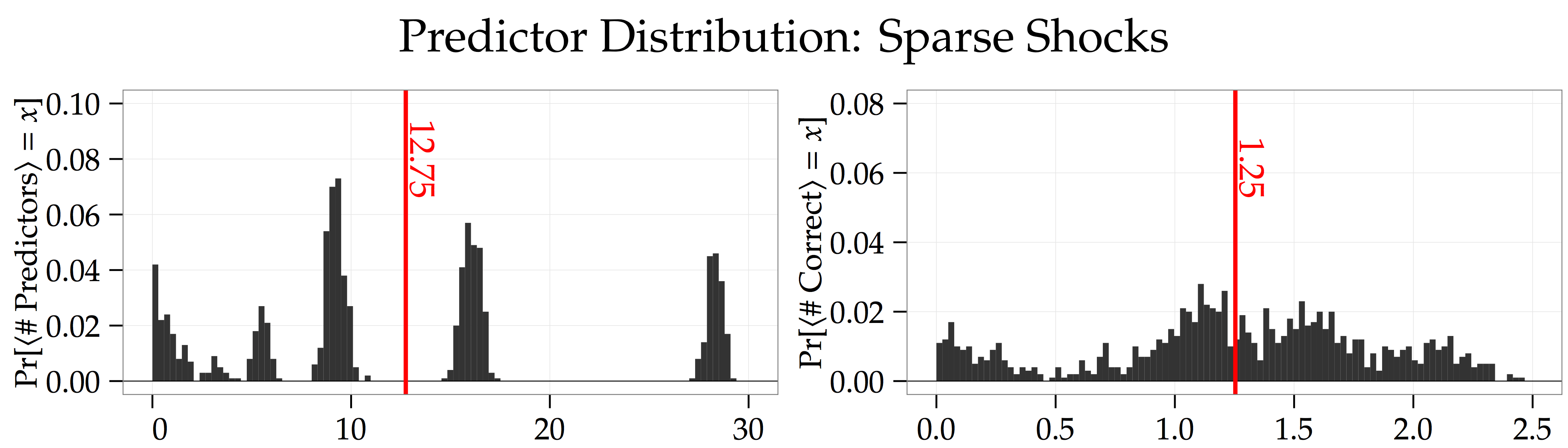
In the second setting, there are too many shocks: $K =75$ . The figures below show that, in both these settings, the LASSO doesn’t add any forecasting power. Thus, running these simulations offers a pair of nice placebo tests showing that the LASSO really is picking up sparse signals in the cross-section of returns.

Notes on Kyle (1989)

November 13, 2015 by Alex

1. Motivating Example

In several earlier posts (e.g., here and here) I’ve talked about the two well-known information-based asset-pricing models, Grossman and Stiglitz (1980) and Kyle (1985). But, there are lots of situations that don’t really fit with either of these two models. For one thing, uninformed speculators often recognize that they’re going to have a price impact, so it’s at odds with Grossman and Stiglitz (1980). For another thing, uninformed speculators typically use limit orders, so it’s at odds with Kyle (1985).

This post outlines the Kyle (1989) model which studies speculators that place limit orders and recognize their own price impact.

2. Market Structure

Assets. There is a single trading period and a single risky asset with a price of $p$ . This risky asset’s liquidation value is $v \sim \mathrm{N}(0, \, \tau_v^{-1})$ . For example, you might think about the asset as a stock that’ll have a value of $v$ after some important news announcement tomorrow. It’s just that, right now, you don’t know which direction the news will go.

Traders. There are $3$ kinds of traders: noise traders, informed speculators, and uninformed speculators. Noise traders demand $-z \sim \mathrm{N}(0, \, \tau_z^{-1})$ shares of the risky asset. There are $N$ informed speculators and $M$ uninformed speculators. Both informed and uninformed traders have an initial endowment of $\mathdollar 0$ (this is just a normalization) and exponential utility with risk-aversion parameter $\rho > 0$ ,

(1) $\begin{align*} - \, \exp\left\{ \, - \, \rho \cdot (v - p) \cdot x \, \right\}, \end{align*}$

where $x$ denotes the number of shares demanded by a speculator.

Information. Prior to trading, each informed speculator gets a private signal $s_n$ and has a demand schedule $\mathrm{X}_{I,n}(p,\,s_n)$ . That is, he has in mind a function which tells him how many shares to demand at each possible price, $p$ , given his private signal, $s_n$ . Assume that the informed speculators’ signals can be written as

(2) $\begin{align*} s_n = v + \epsilon_n \end{align*}$

where $\epsilon_n \sim \mathrm{N}(0, \, \tau_{\epsilon}^{-1})$ . Each uninformed speculator has a demand schedule $\mathrm{X}_{U,m}(p)$ .

3. Equilibrium Concept

Definition. An equilibrium is a set of demand schedules, $X_{I,n}(p,\,s_n)$ for the $n=1,\,2,\,\ldots,\,N$ informed speculators and $X_{U,m}(p)$ for the $m=1,\,2,\,\ldots,\,M$ uninformed speculators, and a price function $P(v,\,z)$ such that (a) markets clear,

(3) $\begin{align*} z &= {\textstyle \sum_{n=1}^N} X_{I,n}(p,\,s_n) + {\textstyle \sum_{m=1}^M} \cdot X_{U,m}(p), \end{align*}$

and (b) both informed and uninformed speculators optimize,

(4) $\begin{align*} X_{I,n}(p,\,s_n) &\in \arg \max_x \left\{ \, \mathrm{E}[ \, - \, \exp\left\{ \, \rho \cdot (v - p) \cdot x \right\} \, | \, p, \, s_n \, ] \, \right\} \text{ for all } n = 1, \, 2, \, \ldots, \, N \\ \text{and} \qquad X_{U,m}(p) &\in \arg \max_x \left\{ \, \mathrm{E}[ \, - \, \exp\left\{ \, \rho \cdot (v - p) \cdot x \right\} \, | \, p \, ] \, \right\} \text{ for all } m = 1, \, 2, \, \ldots, \, M. \end{align*}$

Both informed and uninformed speculators understand the relationship between prices and the random variables $v$ and $z$ . Prices will not be fully revealing due to the presence of noise-trader demand, $z$ .

Refinements. I make a pair of additional restrictions on the set of equilibria. Namely, I look only for linear, symmetric equilibria where the informed speculators’ demand schedules can be written as

(5) $\begin{align*} \mathrm{X}_I(p,\, s_n) &= \alpha_I - \beta_I \cdot p + \gamma_I \cdot s_n, \end{align*}$

the uninformed-speculators’ demand schedules can be written as

(6) $\begin{align*} \mathrm{X}_U(p) &= \alpha_U - \beta_U \cdot p, \end{align*}$

and the price can be written as

(7) $\begin{align*} \mathrm{P}(v,\,z) &= \theta_0 + \theta_v \cdot v - \theta_z \cdot z. \end{align*}$

4. Information Updating

Price Impact. If we substitute the linear demand schedules for the informed and uninformed speculators into the market-clearing condition, then we get a formula for the price,

(8) $\begin{align*} p &= \lambda \times \left( \, \left\{ \, N \cdot \alpha_I + M \cdot \alpha_U \, \right\} + \gamma_I \cdot {\textstyle \sum_{n=1}^N} s_n - z \, \right) \quad \text{where} \quad \lambda = {\textstyle \frac{1}{N \cdot \beta_I + M \cdot \beta_U}}. \end{align*}$

Thus, if noise traders supply one additional share, then the price drops by $\mathdollar \lambda$ . Next, I define the same object for informed and uninformed speculators. That is, taking the demand schedules of the other speculators as given, how much will the price change if the $n$ th informed speculator or $m$ th uninformed speculator increases his demand by $1$ share? This question defines the residual supply curves,

(9) $\begin{align*} p &= \hat{p}_{I,n} + \lambda_I \times X_I(p,\,s_n) \\ \text{and} \qquad p &= \hat{p}_{U} + \lambda_U \times X_U(p). \end{align*}$

Imperfect competition is present because each trader recognizes that if he submits a different schedule, the resulting equilibrium price may change.

Forecast Precision. Informed speculator’s forecast precision is given via Bayesian updating as:

(10) $\begin{align*} \tau_I = \left( \, \mathrm{Var}[v|p,\, s_n] \, \right)^{-1} = \tau_v + \tau_{\epsilon} + \varphi_I \times (N-1) \cdot \tau_{\epsilon} \quad \text{where} \quad \varphi_I = {\textstyle \frac{(N - 1) \cdot \gamma_I^2 \cdot \tau_z}{(N - 1) \cdot \gamma_I^2 \cdot \tau_z + \tau_{\epsilon}}}. \end{align*}$

$\varphi_I$ represents the fraction of the precision from the other $(N-1)$ informed speculators revealed to the $n$ th informed speculator by the price. The corresponding forecast precision for uninformed speculator is:

(11) $\begin{align*} \tau_U = \left( \, \mathrm{Var}[v|p] \, \right)^{-1} = \tau_v + \varphi_U \times N \cdot \tau_{\epsilon} \quad \text{where} \quad \varphi_U = {\textstyle \frac{N \cdot \gamma_I^2 \cdot \tau_z}{N \cdot \gamma_I^2 \cdot \tau_z + \tau_{\epsilon}}}. \end{align*}$

$\varphi_U$ represents the fraction of the precision of the $N$ informed speculators revealed to the $m$ th uninformed speculator by the price. Clearly, prices become perfectly revealing as $\varphi_I, \, \varphi_U \to 1$ .

Posterior Beliefs. The $n$ th informed speculator’s posterior beliefs about the risky asset’s liquidation value is a weighted average of the public price signal and his private signal,

(12) $\begin{align*} \mathrm{E}[v|p, \, s_n] &= \left( {\textstyle \frac{\varphi_I }{\tau_I} \cdot \frac{\tau_{\epsilon}}{\gamma_I}} \right) \times \left( \, \lambda^{-1} \cdot p - \{N \cdot \alpha_I + M \cdot \alpha_U\} \, \right) + \left( {\textstyle \frac{(1 - \varphi_I) \cdot \gamma_I}{\tau_I} \cdot \frac{\tau_{\epsilon}}{\gamma_I}} \right) \times s_n \end{align*}$

Uninformed speculators form their posterior beliefs solely on the public price signal,

(13) $\begin{align*} \mathrm{E}[v|p] &= \left( {\textstyle \frac{\varphi_U}{\tau_U} \cdot \frac{\tau_{\epsilon}}{\gamma_I}} \right) \times \left( \, \lambda^{-1} \cdot p - \{N \cdot \alpha_I + M \cdot \alpha_U\} \, \right). \end{align*}$

5. Optimal Demand

Informed Demand. The $n$ th informed speculator observes his private signal, $s_n$ , and the price implied by the demand of the other traders, $\hat{p}_{I,n}$ . He then solves the optimization problem below,

(14) $\begin{align*} \max_x \left\{ \, (\mathrm{E}[v|\hat{p}_{I,n}, \, s_n] - \hat{p}_{I,n}) \cdot x - (\lambda_I + {\textstyle \frac{\rho}{2}} \cdot \mathrm{Var}[v|\hat{p}_{I,n}, \, s_n]) \cdot x^2 \, \right\} \quad \Rightarrow \quad x = {\textstyle \frac{\mathrm{E}[v|\hat{p}_{I,n}, \, s_n] - \hat{p}_{I,n}}{2 \cdot \lambda_I + \rho \cdot \mathrm{Var}[v|\hat{p}_{I,n}, \, s_n]}}. \end{align*}$

But, the residual demand curve, $\hat{p}_{I,n}$ , is related to the actual price, $\hat{p}_{I,n} = p - \lambda_I \cdot X_I(p,\,s_n)$ . So, after a little bit of rearranging, we can write the informed speculators’ optimal demand schedules as

(15) $\begin{align*} X_I(p,\,s_n) &= {\textstyle \frac{\mathrm{E}[v|p, \, s_n] - p}{\lambda_I + \sfrac{\rho}{\tau_I}}}. \end{align*}$

Uninformed Demand. The $m$ th uninformed speculator observes only the price implied by the demand of the other traders, $\hat{p}_U$ . He then solves the optimization problem below,

(16) $\begin{align*} \max_x \left\{ \, (\mathrm{E}[v|\hat{p}_U] - \hat{p}_U) \cdot x - (\lambda_U + {\textstyle \frac{\rho}{2}} \cdot \mathrm{Var}[v|\hat{p}_U]) \cdot x^2 \, \right\} \quad \Rightarrow \quad x = {\textstyle \frac{\mathrm{E}[v|\hat{p}_U] - \hat{p}_U}{2 \cdot \lambda_U + \rho \cdot \mathrm{Var}[v|\hat{p}_U]}}. \end{align*}$

Using the exact same tricks, we can write the uninformed speculators’ optimal demand schedule as

(17) $\begin{align*} X_U(p) &= {\textstyle \frac{\mathrm{E}[v|p] - p}{\lambda_U + \sfrac{\rho}{\tau_U}}}. \end{align*}$

6. Endogenous Parameters

Next, it’s useful to define a couple of additional parameters.

Information Incidence. First, define the information incidence as

(18) $\begin{align*} \zeta &= \left( {\textstyle \frac{\tau_\epsilon}{\tau_I}} \right)^{-1} \times (\lambda \cdot \gamma_I). \end{align*}$

This new parameter represents the increase in the equilibrium price when the $n$ th informed speculator’s valuation of the risky asset goes up by $\mathdollar 1$ as a result of a higher signal realization, $s_n$ . For trader $n$ ‘s valuation to rise by $\mathdollar 1$ , his private signal must rise by a factor of $(\frac{\tau_\epsilon}{\tau_I})^{-1}$ , and prices move by a factor of $(\lambda \cdot \gamma_I)$ for every $\mathdollar 1$ increase in the $n$ th informed speculator’s private signal, $s_n$ . In equilibrium, it turns out that $\zeta \leq \sfrac{1}{2}$ .

Marginal Market Share. Next, define two parameters capturing the marginal market share of the informed and uninformed speculators,

(19) $\begin{align*} \xi_I = \beta_I \cdot \lambda \quad \text{and} \quad \xi_U = \beta_U \cdot \lambda. \end{align*}$

Here’s how you interpret $\xi_I$ : if noise traders demand $1$ additional share, then the quantity traded by each informed speculator increases by $\xi_I$ shares. Likewise, $\xi_U$ captures the amount of additional trading that each uninformed speculator does in response to a $1$ share increase in noise-trader demand.

7. Model Solution

Kyle (1989) shows that there exists a unique symmetric linear equilibrium if $N \geq 2$ , $M \geq 1$ , $\tau_z^{-1} > 0$ , and $\tau_{\epsilon} > 0$ . This equilibrium is characterized by a system of $4$ equations and $4$ unknowns, $\{ \, \gamma_I, \, \zeta, \, \xi_I, \, \xi_U \, \}$ , subject to the constraints that $\gamma_I > 0$ , $0 < \zeta \leq \sfrac{1}{2}$ , $\sfrac{\varphi_U}{N} < \beta_I \cdot \lambda < \sfrac{1}{N}$ , and $0 < \beta_U \cdot \lambda < \sfrac{(1 - \varphi_U)}{M}$ .

Equation 1. The first equation is the easiest. If noise traders demand an additional share, then someone has to sell it to them. Informed speculators tend to adjust their demand by $\xi_I$ shares, and uninformed speculators tend to adjust their demand by $\xi_U$ shares. Thus, because there are $N$ informed speculators and $M$ uninformed speculators, we have the market-clearing condition below:

(20) $\begin{align*} 1 &= N \cdot \xi_I + M \cdot \xi_U. \end{align*}$

Equation 2. Next, we turn to the second equation, which characterizes the informed speculator’s demand response to price changes, $\beta_I$ , via the endogenous parameter $\xi_I$ ,

(21) $\begin{align*} (1 - \zeta) &= (1 - \varphi_I) \times (1 - \xi_I). \end{align*}$

This equation links how unresponsive prices are to a $\mathdollar 1$ increase in an informed speculator’s private signal, $(1 - \zeta)$ , to the product of how uninformative prices are about other informed speculators’ signals, $(1 - \varphi_I)$ , and how little each informed speculator has to trade in response to a $1$ share increase in noise-trader demand, $(1 - \xi_I)$ . After all, if informed speculators don’t have to trade that often—i.e., $(1 - \xi_I) \approx 1$ —and prices don’t really reveal much of their private signal to other informed speculators when they do—i.e., $(1 - \varphi_I) \approx 1$ , then prices shouldn’t be moving that much in response to private shocks—i.e., $(1 - \zeta) \approx 1$ .

Equation 3. The third equation is much more directly an equilibrium characterization of $\gamma_I$ ,

(22) $\begin{align*} \gamma_I &= \tau_{\epsilon} \times \left( {\textstyle \frac{1}{\rho}} \right) \times (1 - \varphi_I) \times \left( {\textstyle \frac{1 - 2 \cdot \zeta}{1 - \zeta}} \right). \end{align*}$

Informed speculators are going to trade more aggressively in response to a $\mathdollar 1$ increase in their private signal when their private signal is more precise (i.e., $\tau_{\epsilon}$ is big), when they are closer to risk neutral (i.e., $\rho$ is small), when prices don’t reveal much about their private signal to other informed speculators (i.e., $(1 - \varphi_I) \approx 1$ because $\varphi_I \approx 0$ ), or when prices don’t move much when informed speculators trade on their private information (i.e., $\frac{1 - 2 \cdot \zeta}{1 - \zeta} \approx 1$ because $\zeta \approx 0$ ). Notice that this last effect is second order when $\zeta$ is small.

Equation 4. Finally, let’s have a look at equation, which characterizes the uninformed speculator’s demand response to price changes, $\beta_U$ , via the endogenous parameter $\xi_U$ ,

(23) $\begin{align*} \zeta \cdot \tau_U - \varphi_U \cdot \tau_I &= \xi_U \times \underset{> 0}{\left( {\textstyle \frac{\zeta \cdot \tau_U}{1 - \xi_U}} + {\textstyle \frac{\rho \cdot \gamma_I \cdot \tau_I}{\tau_{\epsilon}}} \right)}. \end{align*}$

I don’t have any clean way to analyze the right-hand side of this equation, but it is possible to show that the right-hand side will only be $0$ if $\xi_U = 0$ —that is, if there are lots of small uninformed speculators. What’s more, we know from Equation (13) that prices will only be an unbiased estimate of the uninformed speculators’ beliefs if:

(24) $\begin{align*} 1 &= \left( {\textstyle \frac{\varphi_U \cdot \tau_{\epsilon}}{\gamma_I \cdot \tau_U}} \right) \times \lambda^{-1}. \end{align*}$

If we rearrange the left-hand side of the equation a bit,

(25) $\begin{align*} 0 &= \zeta \cdot \tau_U - \varphi_U \cdot \tau_I \\ \varphi_U \cdot \tau_I &= \zeta \cdot \tau_U \\ \varphi_U \cdot \tau_I &= \left( {\textstyle \frac{\tau_\epsilon}{\tau_I}} \right)^{-1} \cdot (\lambda \cdot \gamma_I) \cdot \tau_U \\ \left( {\textstyle \frac{\varphi_U \cdot \tau_{\epsilon}}{\gamma_I \cdot \tau_U}} \right) \times \lambda^{-1} &= 1, \end{align*}$

we see that prices can only be unbiased if there are lots of small uninformed speculators, just like in Grossman and Stiglitz (1980). Otherwise, prices overreact—that is, $\theta = \left( {\textstyle \frac{\varphi_U \cdot \tau_{\epsilon}}{\gamma_I \cdot \tau_U}} \right) \times \lambda^{-1} < 1$ .

8. Numerical Analysis

To make sure that I’ve understood how to solve the model correctly, I solved for the equilibrium parameters numerically when $\rho=1$ , $N=2$ , $M=1$ , $\tau_{\epsilon}=2$ , and $\tau_v=1$ as the precision of noise-trader demand volatility ranges from $\tau_z = 0$ to $\tau_z = 2$ . You can find the code here. I’ve plotted some of the results below.

Screening Using False-Discovery Rates

November 5, 2015 by Alex

1. Motivating Example

Jegadeesh and Titman (1993) show that, if you rank stocks according to their returns over the previous $12$ months, then the past winners will outperform the past losers by $1.5{\scriptstyle \%}$ per month over the next $3$ months. But, the authors don’t just test this particular strategy. They also test strategies that rank stocks over the previous $3$ , $6$ , and $9$ months and strategies which hold stocks for the next $6$ , $9$ , and $12$ months, too. Clearly, if they test enough hypotheses, then some of these tests are going to appear statistically significant by pure chance. To address this concern in the original paper, the authors use the Bonferroni method.

This post shows how to use an alternative method—namely, controlling the false-discovery rate—to identify statistically significant results when testing multiple hypotheses.

2. Bonferroni Method

First, here’s the logic behind the Bonferroni method. Suppose you want to run $N \gg 1$ different hypothesis tests, $\{ \, h_1, \, h_2, \, \ldots, \, h_N \, \}$ . Let $h_n = 0$ if the $n$ th null hypothesis is true and $h_n = 1$ if the $n$ th null hypothesis is false (i.e., should be rejected). Let $p_n$ denote the p-value associated with some test statistic for the $n$ th hypothesis. If there were just one test, then we should simply reject the null whenever $p_1 \leq 0.05$ . But, if there are many tests, then this no longer works. If you look at a lot of hypotheses, then $5{\scriptstyle \%}$ of the p-values should be less than $0.05$ even if $h_n = 0$ for all of them. The Bonferroni method suggests correcting this problem by lowering the p-value associated with the $5{\scriptstyle \%}$ significance level and only rejecting the null hypothesis when

(1) $\begin{align*} p_n \leq {\textstyle \frac{1}{N}} \cdot 0.05. \end{align*}$

i.e., if there are $N = 10$ hypothesis tests, then only reject the null at the $5{\scriptstyle \%}$ significance level when the p-value is less than $0.005$ rather than $0.05$ .

This is a nice start, but it turns out that the Bonferroni method is way too strict. Imagine drawing samples of $10$ observations from $N$ different normal distributions. All samples have the same standard deviation, $\sigma = 1$ , but not all of the sample have the same mean. $20{\scriptstyle \%}$ have a mean of $\mu = 1$ , and the rest have a mean of $\mu = 0$ . The figure below shows that, if we use the Bonferroni method to identify which of the $N = 100$ samples have a non-zero mean, then we’re only going to choose $2$ samples. But, by construction, we know that $20$ samples had a non-zero mean! We should be rejecting the null $10$ -times more often!

3. False-Discovery Rate

Now, let’s talk about false-discovery rates. Define $R(0.05) = \sum_{n=1}^N 1_{\{p_n < 0.05\}}$ as the total number hypotheses that you reject at the $5{\scriptstyle \%}$ significance level. Similarly, define $R_f(0.05) = \sum_{n=1}^N 1_{\{p_n < 0.05\}} \times 1_{\{ h_n = 0 \}}$ as the number of hypotheses that you reject at the $5{\scriptstyle \%}$ significance level where the null was actually true—i.e., these are false rejections. The false-discovery rate is then

(2) $\begin{align*} \mathit{FDR} = \mathrm{E}\left[ \, \sfrac{R_f}{R} \, \right]. \end{align*}$

Let’s return to the numerical example above to clarify this definition. Suppose we had a test that identified all $20$ cases where the sample mean was $\mu = 1$ , $R = 20$ . If we wanted a false-discovery rate $\mathit{FDR} \leq 0.10$ , then this test could produce at most $2$ false rejections, $R_f \leq 2$ . If the test identified only half of the $20$ cases where the sample mean was $\mu =1$ , $R = 10$ , then this test could produce at most $1$ one false rejection, $R_f \leq 1$ .

Benjamini and Hochberg (1995) first introduced the idea that you could use the false-discovery rate to adjust statistical-significance tests when exploring multiple hypotheses. Here’s their recipe. First, run all of your tests and order the resulting p-values,

(3) $\begin{align*} p_{(1)} \leq p_{(2)} \leq \cdots \leq p_{(n)} \leq \cdots \leq p_{(N)}. \end{align*}$

Then, for a given false-discovery rate, $x$ , define $n_x$ as

(4) $\begin{align*} n_x = \max_{n \in N} \, \left\{ \, n \, : \, p_{(n)} \leq {\textstyle \frac{n}{N} \cdot x} \, \right\}. \end{align*}$

Benjamini and Hochberg (1995) showed that, if you reject any null hypothesis where

(5) $\begin{align*} p_n \leq p_{(n_x)}, \end{align*}$

then $\mathit{FDR} \leq x$ , guaranteed. If we apply the false-discovery-rate procedure to the same numerical example from above using the $x = 0.05$ threshold, then we see that as the number of hypotheses gets large, $N \to \infty$ , the fraction of rejected null hypotheses hovers around $0.06$ . Improvement! It’s no longer shrinking to $0$ . Notice that neither method allows us to pick out the full $20{\scriptstyle \%}$ of null hypotheses that should be rejected in the simulation.

4. Why’s This So?

It’s pretty clear how the Bonferroni method works. If there are lots of hypotheses and you are worried about rejecting the null by pure chance, then just make it harder to reject the null. i.e., lower the threshold for significant p-values. It’s much less clear, though, how the false-discovery-rate screening process works. All you get is a recipe and a guarantee. If you do the list of things prescribed by Benjamini and Hochberg (1995), then you’ll falsely reject no more than $x{\scriptstyle \%}$ of your null hypotheses. Let’s explore the proof of this result from Storey, Taylor and Siegmund (2003) to better understand where this guarantee comes from.

What does it mean to have a useful test? Well, if $h_n = 0$ (null is true), then $p_n$ is drawn randomly from a uniform distribution, $\mathrm{U}(0,\,1)$ . However, if you have a useful test statistic, then if $h_n = 1$ (null is false), then $p_n$ is drawn from some other distribution, $\mathrm{A}(0,\,1)$ that is more concentrated around $0$ . The distribution of p-values is then given by

(6) $\begin{align*} \mathrm{G} = \pi \cdot \mathrm{U} + (1 - \pi) \cdot \mathrm{A}. \end{align*}$

If we reject all p-value less than $x$ , then with a little bit of algebra we can see that

(7) $\begin{align*} \mathit{FDR}(x) = \mathrm{E}\left[ \, \frac{ {\textstyle \sum_{n=1}^N} 1_{\{ p_n \leq x\}} \times 1_{\{ h_n = 0 \}} }{ {\textstyle \sum_{n=1}^N} 1_{\{ p_n \leq x \}} } \, \right] &= \frac{ \mathrm{E}\left[ \, {\textstyle \sum_{n=1}^N} 1_{\{ p_n \leq x\}} \times 1_{\{ h_n = 0 \}} \, \right] }{ \mathrm{E}\left[ \, {\textstyle \sum_{n=1}^N} 1_{\{ p_n \leq x \}} \, \right] } + \mathrm{O}\left( {\textstyle \frac{1}{\sqrt{N}}} \right) \\ &= \frac{ N \cdot \mathrm{Pr}( p_n \leq x | h_n = 0 ) \cdot \mathrm{Pr}(h_n = 0) }{ N \cdot \mathrm{G}(x) } + \mathrm{O}\left( {\textstyle \frac{1}{\sqrt{N}}} \right) \end{align*}$

where the last step uses the fact that $R(x) = {\textstyle \sum_{n=1}^N} 1_{\{ p_n \leq x \}} = N \cdot \mathrm{G}(x)$ and $\mathrm{O}( \sfrac{1}{\sqrt{N}})$ denotes “big-O” notation. Since p-values are drawn from a uniform distribution when the null hypothesis is true, we know that $x = \mathrm{Pr}( p_n \leq x | h_n = 0 )$ . Thus, we can simplify even further:

(8) $\begin{align*} \mathit{FDR}(x) &= \frac{ x \cdot \mathrm{Pr}(h_n = 0) }{ \mathrm{G}(x) } + \mathrm{O}\left( {\textstyle \frac{1}{\sqrt{N}}} \right). \end{align*}$

Now comes the trick. $x$ can be anything we want between $0$ and $1$ . So, let’s choose $x$ as one of the ordered p-values, $p_{(n)}$ . If we do this, then $\mathrm{G}(p_{(n)}) = \sfrac{n}{N}$ and

(9) $\begin{align*} \mathit{FDR}(p_{(n)}) \approx \frac{p_{(n)} \cdot \mathrm{Pr}(h_n = 0) \cdot N}{n} \leq \frac{p_{(n)} \cdot N}{n}. \end{align*}$

If we set the right-hand side equal to the false-discovery-rate tolerance, $0.05$ , and solve for $p_{(n)}$ , then we get the threshold value for $p_{(n)}$ in Benjamini and Hochberg (1995),

(10) $\begin{align*} p_{(n)} = {\textstyle \frac{n}{N}} \times 0.05. \end{align*}$

If we only reject hypotheses where $p_n \leq {\textstyle \frac{n}{N}} \times 0.05$ , then our false-discovery rate is capped at $5{\scriptstyle \%}$ .

Persistence and Dispersion in the Housing Market

September 29, 2015 by Alex

1. Motivation

House-price growth is persistent. When you regress current house-price growth on lagged house-price growth using monthly Zip-code level data,

(1) $\begin{align*} \Delta \bar{p}_{z,t} &= \alpha_z + \beta_z \cdot \Delta \bar{p}_{z,t-1} + \varepsilon_{z,t}, \end{align*}$

you find positive predictive power, $\langle \beta_z \rangle > 0$ . Using MSA- or county-level data gives similar results. If prices were growing faster than usual last month, then they’ll be growing faster than usual next month as well.

This persistence shouldn’t exist in a fully rational model with no frictions. Obviously, people aren’t necessarily fully rational and the housing market isn’t frictionless, but exactly which distortions are important for explaining the persistence in house-price growth? There’s been a lot of research trying to answer this question. People have “explained” the persistence in house-price growth using models with naive search/learning (Head, Lloyd-Ellis, and Sun (2013)), extrapolative beliefs (Glaeser and Nathanson (2015)), and lending frictions (Stein (1995) and Glaeser, Gottlieb, and Gyourko (2013)) to give just a few examples. By any reasonable count, there are now more answers than there are questions.

In a new working paper [link], Aurel Hizmo and I present a new stylized fact—namely, that it’s the places with the most homogeneous housing stock have the most persistent house-price growth—which helps discriminate between some of the many plausible explanations above. We find that Zip codes like 90713 (Lakewood, CA), where all the houses are really similar to one another, have very persistent house-price growth; whereas, Zip codes like 90402 (Santa Monica, CA), where the housing stock is really heterogeneous, have less persistent house-price growth. This fact suggests that naive search/learning, explanations which rely on house-to-house variation in quality, are unlikely to be key drivers of price-growth persistence. In this post, I outline a simple economic model to make this intuition more concrete: if naive search/learning is causing price-growth persistence, then it should be the places with the most heterogeneous housing stock that have the most persistent price growth.

2. House Values

Let’s study a Zip-code-level housing market with an aggregate supply of $\psi$ houses. Let $\bar{v}_T$ denote the average value of owning a home in this Zip code at time $T$ . Think about this as the consumption dividend from living in a randomly selected home in that Zip code. Suppose that this dividend is the sum of a whole bunch of independent Zip-code-level shocks,

(2) $\begin{align*} \bar{v}_T &= \bar{v}_0 + {\textstyle \sum_{t=1}^T} \, \bar{\epsilon}_t, \end{align*}$

with $\bar{\epsilon}_t \overset{\scriptscriptstyle \mathrm{iid}}{\sim} \mathrm{N}(0, \, \sigma_{\epsilon}^2)$ . For example, one month a park might get built (a positive shock), the next month a nearby grocery store might close (a negative shock), and so on… In the analysis below, I use the $\bar{x}$ notation to denote the Zip-code-level average of $x$ , where $x$ is any arbitrary variable in the model.

Now, suppose that within the Zip code there are $K$ different kinds of houses. For instance, if you’re thinking about Lakewood, CA where all the houses are identical, then $K=1$ . By contrast, if you’re thinking about Santa Monica, CA where the housing stock is very heterogeneous, then $K \gg 1$ . Each aggregate Zip-code-level shock is the average of the shocks to each of the $K$ housing types,

(3) $\begin{align*} \bar{\epsilon}_t &= {\textstyle \frac{1}{K} \cdot \sum_{k=1}^K} \, \epsilon_{k,t}, \end{align*}$

with $\epsilon_{k,t} \sim \mathrm{N}(0, \, K \cdot \sigma_{\epsilon}^2)$ . For example, the grocery-storing-closing shock might be a really negative shock for the part of the Zip code closest to the store, but only a minor inconvenience for the part of the Zip code farthest from the store who only shopped there occasionally.

3. Information Structure

Next, let’s turn our attention to the information structure in the model. We want to capture the idea that it’s more difficult to learn about how awesome it would be to live in a Zip code if the housing stock is more heterogeneous. After all, if you’ve seen one house in Lakewood, CA, then you’ve seen them all. By contrast, the first house you see in Santa Monica, CA might not be very representative of what it’s like to live there since all the houses are so different.

Here’s how the information structure works. There’s a unit mass of buyers and that each buyer can only view one kind of house each period. At time $t$ , buyers begin seeing signals about, $\bar{\epsilon}_{[t-1]+K}$ , that is, the Zip-code-level shock that will occur at time $([t-1]+K)$ . But, buyers don’t get to see the full shock right away. A randomly selected group of $\sfrac{1}{K}$ buyers will see the signal for the first kind of house, $\epsilon_{1,[t-1]+K}$ , another randomly selected group of $\sfrac{1}{K}$ buyers will see the signal for the second kind of house, $\epsilon_{2,[t-1]+K}$ , and so on… until the $K$ th group of $\sfrac{1}{K}$ buyers sees the signal for the $K$ th kind of house, $\epsilon_{K,[t-1]+K}$ . So, each of the signals about the Zip code’s time $([t-1]+K)$ shock will been seen by $(\sfrac{1}{K})$ th of the buyers at time $t$ . You can think about this as buyer shopping around and each seeing different kinds of houses. After seeing their initial signals, each buyer can then form posterior beliefs about the value of owning a house in that Zip code.

At time $(t+1)$ , the same process then repeats with each buyer viewing the time $([t-1]+K)$ signal for a different kind of house. A randomly selected group of $\sfrac{1}{K}$ buyers who haven’t already looked at the first kind of house will see the signal for the first kind of house, $\epsilon_{1,[t-1]+K}$ , another randomly selected group of $\sfrac{1}{K}$ buyers who haven’t already looked at the second kind of house will see the signal for the second kind of house, $\epsilon_{2,[t-1]+K}$ , and so on… until a $K$ th group of $\sfrac{1}{K}$ buyers that hasn’t already looked at the $K$ th kind of house sees the signal for the $K$ th kind of houses, $\epsilon_{K,[t-1]+K}$ . So, each of the signals about the Zip code’s time $([t-1]+K)$ shock will been seen by $(\sfrac{2}{K})$ th of the buyers at time $(t+1)$ . This learning process keeps on going until all buyers have seen all signals for the time $([t-1]+K)$ Zip-code-level shock by the end of period $([t-1]+K)$ .

This information structure is analytically convenient because it makes sure that each buyer has seen the same amount of information at each point in time, even though no $2$ buyers will have seen the same signals. So, the parameter $K$ can be thought of as a proxy for information flow or the rate of learning. Larger values of $K$ mean that it takes buyers longer to learn about the Zip code’s fundamental value. Note that this setup is formally equivalent to the “rotation” convention used in Hong and Stein (1999).

4. Buyer Preferences

Finally, to complete the model, let’s have a look at the home-buyers’ preferences. I assume that buyers have constant-absolute–risk-aversion (CARA) utility with risk-aversion parameter, $\rho > 0$ . Each period buyers choose how many shares of housing to buy in the Zip code, $x_{b,t}$ , and how many shares of the riskless asset to buy, $y_{b,t}$ , in order to maximize their time $T$ wealth, $w_{b,T}$ ,

(4) $\begin{align*} \max_{(x_{b,t}, \, y_{b,t})_{t=1}^T} \, \mathrm{E}_{b,t}[ \, - \exp\{ \, - \rho \cdot w_{b,T} \, \} \, ] \quad \text{s.t.} \quad w_0 \geq \bar{p}_t \cdot x_{b,t} + y_{b,t}. \end{align*}$

I normalize the net riskless rate is $r_f = 0$ .

For simplicity, let’s assume that at every time, $t$ , the buyers formulate their housing demand based on the static-optimization notion that they’re going to buy and hold until time $T$ . This’ll make the pricing equations really clean and won’t affect the intuition. However, to be clear, it does introduce an element of time inconsistency. Although home buyers formulate their time $t$ demand based on the assumption that they won’t re-trade, they violate this assumption if they are active in later periods.

5. Fully-Rational Equilibrium

With the model in place, we can now turn our attention to the solution. First, let’s study the fully-rational equilibrium as a benchmark case. If each buyer recognizes that the market-clearing price reveals information about the set of signals that the other buyers got, then, by the logic of Grossman (1976), prices should be fully revealing because there is no uncertainty about housing supply,

(5) $\begin{align*} \bar{p}_t^{\text{rational}} &= \bar{v}_{[t-1]+K} - \mathrm{f}(\rho) \cdot \psi \\ &= \bar{v}_{t-1} + {\textstyle \sum_{k=0}^{K-1}} \bar{\epsilon}_{t+k} - \mathrm{f}(\rho) \cdot \psi, \end{align*}$

where $\mathrm{f}(\rho)$ is a function of the home buyers’ risk-aversion parameter. This is why you need the random-asset-supply assumption in models like Grossman and Stiglitz (1980) and Hellwig (1980).

Obviously, in this setup there isn’t going to be any price-growth persistence,

(6) $\begin{align*} \mathrm{Cov}[\Delta \bar{p}_t^{\text{rational}}, \, \Delta \bar{p}_{t-1}^{\text{rational}}] = 0, \end{align*}$

because each of the Zip-code-level shocks is drawn independently. This result shows that search/learning on its own is not enough to generate persistence. You need people to be naive as well. You need people to be ignoring some information.

6. Equilibrium with Persistence

Suppose buyers don’t condition on current or past prices. e.g., think about this as an extreme form of a cursed equilibrium as in Eyster, Rabin, and Vayanos (2015) or just as a Walrasian equilibrium with private valuations. In this setting, the Zip-code level house prices will be given by

(7) $\begin{align*} \bar{p}_t^{\text{na\"{i}ve}} &= \bar{v}_{t-1} + {\textstyle \sum_{k=0}^{K-1}} \left({\textstyle \frac{K - k}{K}}\right) \cdot \bar{\epsilon}_{t+k} - \mathrm{f}(\rho) \cdot \psi, \end{align*}$

where again $\mathrm{f}(\rho)$ is a function of buyers’ risk-aversion parameter. Because buyers ignore some information, it takes longer for shocks to fundamentals to work their way into prices. As a result, price movements are now persistent.

Let’s compute the level of persistence to see how it varies with the heterogeneity of the housing stock, $K$ . First, note that changes in the Zip-code-level price are given by:

(8) $\begin{align*} \Delta \bar{p}_t^{\text{na\"{i}ve}} &= {\textstyle \frac{1}{K}} \cdot {\textstyle \sum_{k=0}^{K-1}} \bar{\epsilon}_{t+k}. \end{align*}$

Thus, the level of auto-correlation is given by:

(9) $\begin{align*} \frac{ \mathrm{Cov}[\Delta \bar{p}_t^{\text{na\"{i}ve}}, \, \Delta \bar{p}_{t-1}^{\text{na\"{i}ve}}] }{ \mathrm{Var}[\Delta \bar{p}_{t-1}^{\text{na\"{i}ve}}] } &= \frac{K-1}{K} \end{align*}$

With this formulation, you see that the more heterogeneous the housing stock (i.e., the higher the $K$ ), the more persistent the house-price level will be. After all, house prices are a weighted average of past shocks in this setting. Buyers consistently under-react to new information.

You can write down this sort of naive search/learning model in lots of ways. But, no matter how you do it, you always get this sort of result. When assets are more heterogeneous—that is, when there is more to learn about—price growth is more persistent. Thus, when Aurel and I find that Zip codes with the most homogeneous housing stock have the most price-growth persistence, this is strong evidence that naive search/learning isn’t the explanation. It’s got to be something else like, for example, extrapolative beliefs.

« Previous Page