Alex – Page 8 – Research Notebook

Multiscale Noisy-Rational-Expectations Equilibrium

August 28, 2015 by Alex

1. Motivation

Evolutionarily Slow. In modern financial markets, people simultaneously trade the exact same assets on vastly different timescales. For example, a Jegadeesh and Titman (1993)-style momentum portfolio turns over half its holdings once every $6$ months. By contrast, Kirilenko, Kyle, Samadi, and Tuzun (2014) estimate that “high-frequency traders (HFTs) reduce half of their net holdings in $137$ seconds.” These two horizons differ by $5$ orders of magnitude:

(1) $\begin{align*} \frac{\sfrac{1}{2} \, {\scriptstyle \mathrm{holdings}}}{137 \, {\scriptstyle \mathrm{seconds}}} \times \frac{60 \, {\scriptstyle \mathrm{seconds}}}{1 \, {\scriptstyle \mathrm{minute}}} \times \frac{60 \, {\scriptstyle \mathrm{minutes}}}{1 \, {\scriptstyle \mathrm{hour}}} \times \frac{24 \, {\scriptstyle \mathrm{hours}}}{1 \, {\scriptstyle \mathrm{day}}} \times \frac{30 \, {\scriptstyle \mathrm{days}}}{1 \, {\scriptstyle \mathrm{month}}} \times \frac{6 \, {\scriptstyle \mathrm{months}}}{\sfrac{1}{2} \, {\scriptstyle \mathrm{holdings}}} = 1.1 \times 10^5. \end{align*}$

This is a big number. To put it in perspective, there have only been around $2 \times 10^5$ generations since the human/chimpanzee divergence. See MacKay (2003, C4). So, in a quite literal sense, momentum traders are evolutionarily slow by HFT standards. This difference in timescales has a couple of important implications.

Different Strokes. First, because their respective timescales are so different, short- and long-run traders value assets differently. One reason is purely mechanical: short-run traders have to close out their positions at the end of each day. Why should they be interested in a company’s quarterly cash flows? Another reason is more subtle: a trader’s timescale affects the kind of information he can process. Short-run traders operate at speeds faster than any human can handle, so these traders have to focus on machine-readable information; whereas, long-run traders operate on more human timescales, so these traders tend to focus on soft information. Traders at different timescales also have very different educational backgrounds. As the pace of trading gets faster, traders become more likely to have a background in mathematics, computer science, or engineering than a background in economics, finance, or accounting.

Predictable Demand. Second, because long-run traders’ timescale is so slow, their order flow will look slightly predictable to short-run traders. If long-run traders space their orders out over the course of a month, then demand in the previous minute is going to give short-run traders a little bit of information about what demand will be like in the next minute. The SEC points out in a 2010 report that short-run traders often use “sophisticated pattern recognition software to ascertain from publicly available information the existence of a large buyer (seller)” or “ping different market centers in an attempt to locate and trade in front of large buyers (sellers).” Even if you didn’t know that the last common ancestor we shared with chimpanzees would eventually evolve into humans in the long-run, at each step along the way, you could look at two parents and still have a pretty good idea of what their offspring were going to be like.

What It All Means. These two observations imply that short-run traders will want to adjust their own trading behavior due to the presence of long-run traders and vice versa, affecting the returns we observe at each horizon. Put another way, a pair of assets with the same fundamentals might realize different returns because their traders operate at different timescales. This post outlines an asset-pricing model studying precisely this effect. It’s an overview of the model in my paper, When Fast Trading Looks Like Priced Noise.

2. Market Structure

Long-Run Value. There are $T$ trading periods and a single asset that has a long-run fundamental value of

(2) $\begin{align*} v \sim \mathrm{N}(\mu_v, \, \sigma_v^2). \end{align*}$

For instance, you might think about $v$ as a liquidating dividend. There is the same amount of variance in the long-run fundamental value regardless of the number of trading periods. After all, a factory’s production doesn’t get more erratic if people start to trade shares in the company that owns it more quickly.

Short-Run Value. This asset also realizes short-run, transient, value shocks

(3) $\begin{align*} \epsilon_t \overset{\scriptscriptstyle \mathrm{iid}}{\sim} \mathrm{N}(0, \, \sigma_{\epsilon}^2) \end{align*}$

that are irrelevant in the long-run. For instance, you might think about each $\epsilon_t$ as a payment from an exchange for providing liquidity. Importantly, short-run traders care about both the permanent and the transient parts of an asset’s short-run value when choosing their portfolio holdings,

(4) $\begin{align*} \tilde{v}_t = v + \epsilon_t. \end{align*}$

Algorithmic traders have to close out their positions overnight. So, they can’t justify an awful P&L statement on Monday by telling their MD that holding the position for a month will return it to the black.

Pricing Rule. Each period, uninformed market makers set the asset’s price equal to their conditional expectation of the asset’s long-run fundamental value after observing the aggregate demand for the asset,

(5) $\begin{align*} p_t = \mathrm{E}[v|a_t] = \lambda_0 + \lambda_a \times a_t \qquad \text{with} \qquad a_t = x_t + y + z_t. \end{align*}$

Here, $x_t$ denotes the number of shares bought by the short-run trader, $y$ denotes the number of shares bought by the long-run trader, and $z_t \overset{\scriptscriptstyle \mathrm{iid}}{\sim} \mathrm{N}(0, \, \sigma_z^2)$ denotes the number of shares bought by noise traders.

To offset their expected losses from trading with more informed agents, market makers charge a fee, $\kappa$ , to each group of traders where

(6) $\begin{align*} \kappa &= \mathrm{E}[ \, {\textstyle \frac{1}{\sigma_a} \cdot \sum_{t=1}^T} (v - p_t) \cdot a_t \, ]. \end{align*}$

So, the monthly price we observe in the data is $\hat{p} = (\frac{1}{T} \cdot \sum_{t=1}^T p_t) - \kappa$ . As Brennan and Subrahmanyam (1996) write, “privately informed investors create significant illiquidily costs for uninformed investors, implying that the required rates of return should be higher for securities that are relatively illiquid.” A fee is a simple way of building this price effect into the model. Alternatively, you could add in this price effect by getting rid of the market maker and modeling risk-averse informed traders facing imperfect competition a la Kyle (1989), but this approach leads to a much more complicated analysis without any additional insight.

3. Short-Run Traders

Optimization Problem. There are $T$ groups of short-run traders that each trade in a single period. Because long-run traders trade so gradually compared to short-run traders, their demand will be slightly predictable and, thus, give away some of their private information about long-run fundamentals. So, prior to trading, short-run traders observe not only the combined short-run value of the asset, $\tilde{v}_t$ , but also a signal about the asset’s long-run fundamental value, $s_t$ . These traders then solve the static optimization problem below,

(7) $\begin{align*} \max_{x_t} \, \mathrm{E}\left[ \, (\tilde{v}_t - p_t) \cdot x_t \, \middle| \, \tilde{v}_t, \, s_t \, \right]. \end{align*}$

The short-run traders’ signal each period is centered around the asset’s long-run fundamental value and gets more precise when long-run traders trade more aggressively,

(8) $\begin{align*} s_t &\overset{\scriptscriptstyle \mathrm{iid}}{\sim} \mathrm{N}( v, \, \sfrac{\sigma_z^2}{\gamma_v^2} ), \end{align*}$

where $\gamma_v$ is the long-run traders’ demand response which I define in the next section. So, the more long-run traders act on their private information, the more this information leaks out to short-run traders.

Demand Rule. I look for a linear demand rule:

(9) $\begin{align*} x_t &= \beta_0 + \beta_{\tilde{v}} \times \tilde{v}_t + \beta_s \times s_t. \end{align*}$

The coefficient $\beta_0$ has units of $\mathrm{shares}$ and captures how many shares a short-run trader will demand on average. The coefficient $\beta_{\tilde{v}}$ has units of $\sfrac{(\mathrm{shares})^2\!}{\mathdollar}$ and captures how many additional shares a short-run trader will demand in the current period if the total short-run value increases by $\mathdollar 1$ per share. The coefficient $\beta_s$ also has units of $\sfrac{(\mathrm{shares})^2\!}{\mathdollar}$ but captures how many additional shares a short-run trader will demand if his signal about the long-run fundamental value of the asset gets $\mathdollar 1$ per share more optimistic.

4. Long-Run Traders

Optimization Problem. There is a single group of long-run traders who observe the long-run fundamental value of the asset, $v$ . These traders solve the static optimization problem below,

(10) $\begin{align*} \max_y \, \mathrm{E}\left[ \, {\textstyle \sum_{t=1}^T} (v - p_t) \cdot y \, \middle| \, v \, \right]. \end{align*}$

Long-run traders have to demand the exact same number of shares every single time. This is what makes them “long-run” and why there is no time subscript on their demand, $y$ . For instance, you can think about long-run traders as traders who slowly adjust their positions using instruments like time-weighted average pricing rules, which automatically execute trades over a predetermined timeframe.

Demand Rule. Again, I look for a linear demand rule:

(11) $\begin{align*} y = \gamma_0 + \gamma_v \times v \end{align*}$

The coefficient $\gamma_0$ has units of $\mathrm{shares}$ and captures how many shares the long-run trader will demand on average. The coefficient $\gamma_v$ has units of $\sfrac{(\mathrm{shares})^2\!}{\mathdollar}$ and captures how many additional shares the long-run trader will demand in each trading period if the long-run fundamental value increases by $\mathdollar 1$ per share.

5. Solving the Model

Short-Run Demand. When you account for long-run trader’s demand rule, short-run traders’ problem morphs into:

(12) $\begin{align*} \max_{x_t} \, \mathrm{E}\left[ \, (\tilde{v}_t - \lambda_0 - \lambda_a \cdot \{ x_t + \gamma_0 + \gamma_v \cdot v + z_t\}) \cdot x_t \, \middle| \, \tilde{v}_t, \, s_t \, \right]. \end{align*}$

After observing the combined short-run asset value and their signal about long-run fundamental value, short-run traders have posterior beliefs of

(13) $\begin{align*} \mathrm{E}[v|\tilde{v}_t,s_t] &= \psi \cdot \omega \cdot \mu_v + (1 - \psi) \cdot \omega \cdot \tilde{v}_t + (1 - \omega) \cdot s_t \\ \text{and} \quad \mathrm{Var}[v|\tilde{v}_t,s_t] &= \psi^2 \cdot \omega^2 \cdot \sigma_v^2 + (1 - \psi)^2 \cdot \omega^2 \cdot \sigma_{\epsilon}^2 + (1 - \omega)^2 \cdot {\textstyle \frac{\sigma_z^2}{\gamma_v^2}} \end{align*}$

where $\psi = \sfrac{\sigma_{\epsilon}^2}{(\sigma_v^2 + \sigma_{\epsilon}^2)}$ and $\omega = \sfrac{(\sfrac{\sigma_z^2}{\gamma_v^2})}{(\psi \cdot \sigma_v^2 + \sfrac{\sigma_z^2}{\gamma_v^2})}$ . Thus, the short-run traders’ optimal demand is given by:

(14) $\begin{align*} x_t &= \left( \, - \, {\textstyle \frac{1}{2 \cdot \lambda_a}} \cdot \{ \lambda_0 + \lambda_a \cdot ( \gamma_0 + \gamma_v \cdot \psi \cdot \omega \cdot \mu_v ) \} \, \right) \\ &\qquad \qquad + \, \left( \, {\textstyle \frac{1}{2 \cdot \lambda_a}} \cdot \{ 1 - \lambda_a \cdot \gamma_v \cdot (1 - \psi) \cdot \omega \} \, \right) \times \tilde{v}_t \\ &\qquad \qquad \qquad \qquad + \, \left( \, - \, {\textstyle \frac{\gamma_v}{2}} \cdot (1 - \omega) \, \right) \times s_t. \end{align*}$

Long-Run Demand. When you account for short-run traders’ demand rule, the long-run trader’s problem turns into:

(15) $\begin{align*} \max_y \, \mathrm{E}\Big[ \, T \cdot \Big( \, v - \{ \lambda_0 + \lambda_a \cdot (\beta_0 + \beta_{\tilde{v}} \cdot \underset{=v}{{\textstyle \frac{1}{T} \cdot \sum_{t=1}^T} \tilde{v}_t} + \beta_s \cdot \underset{=v}{{\textstyle \frac{1}{T} \cdot \sum_{t=1}^T} s_t} + y + \underset{=0}{{\textstyle \frac{1}{T} \cdot \sum_{t=1}^T} z_t}) \} \, \Big) \cdot y \, \Big| \, v \, \Big] \end{align*}$

Notice that, as the number of short-run trading periods grows large, $T \nearrow \infty$ , the long-run trader’s problem becomes completely deterministic because they only care about the average price. From the point of view of the long-run trader, transient asset-value fluctuations blur together and average out in the same way that you can’t tell with the naked eye that incandescent lights actually flicker at 60Hz. Thus, the long-run trader’s optimal demand is given by:

(16) $\begin{align*} y &= \left( \, - \, {\textstyle \frac{1}{2 \cdot \lambda_a}} \cdot \{ \lambda_0 + \lambda_a \cdot \beta_0 \} \, \right) + \left( \, {\textstyle \frac{1}{2 \cdot \lambda_a}} \cdot \{ 1 - \lambda_a \cdot (\beta_{\tilde{v}} + \beta_s) \} \, \right) \times v. \end{align*}$

The short-run traders’ demand coefficients still show up in the long-run trader’s demand rule. So, even though all of the short-run, transient, value shocks average out, there are still echoes of the short-run traders’ demand rule in the long-run.

System of Equations. Given the short- and long-run traders’ optimal demand rules, the market maker in each trading period sets the price equal to his conditional expectation of the asset’s long-run fundamental value after observing the aggregate demand:

(17) $\begin{align*} p_t &= \left( \left\{ 1 - \lambda_a \cdot ( \beta_{\tilde{v}} + \beta_s + \gamma_v ) \right\} \cdot \mu_v - \lambda_a \cdot \{\beta_0 + \gamma_0\} \right) + \left( {\textstyle \frac{(\beta_{\tilde{v}} + \beta_s + \gamma_v) \cdot \sigma_v^2}{(\beta_{\tilde{v}} + \beta_s + \gamma_v)^2 \cdot \sigma_v^2 + \beta_{\tilde{v}}^2 \cdot \sigma_{\epsilon}^2 + \{1 + \sfrac{\beta_s^2}{\gamma_v^2}\} \cdot \sigma_z^2}}\right) \times a_t. \end{align*}$

Thus, the equilibrium slope coefficients are defined by the following system of $4$ equations and $4$ unknowns:

(18) $\begin{align*} \beta_{\tilde{v}} &= \phantom{-} {\textstyle \frac{1}{2 \cdot \lambda_a}} \cdot ( 1 - \lambda_a \cdot \gamma_v \cdot (1 - \psi) \cdot \omega ), \\ \beta_s &= - \, \, {\textstyle \frac{\gamma_v}{2}} \, \, \cdot (1 - \omega), \\ \gamma_v &= \phantom{-} {\textstyle \frac{1}{2 \cdot \lambda_a}} \cdot ( 1 - \lambda_a \cdot \{\beta_{\tilde{v}} + \beta_s\} ), \\ \text{and} \qquad \lambda_a &= \phantom{-} {\textstyle \frac{(\beta_{\tilde{v}} + \beta_s + \gamma_v) \cdot \sigma_v^2}{(\beta_{\tilde{v}} + \beta_s + \gamma_v)^2 \cdot \sigma_v^2 + \beta_{\tilde{v}}^2 \cdot \sigma_{\epsilon}^2 + \{1 + \sfrac{\beta_s^2}{\gamma_v^2}\} \cdot \sigma_z^2}}. \end{align*}$

After solving the slop coefficients, the equilibrium level coefficients are then pinned down by a further system of $3$ equations and $3$ unknowns:

(19) $\begin{align*} \beta_0 &= - \, {\textstyle \frac{1}{2 \cdot \lambda_a}} \cdot \{ \lambda_0 + \lambda_a \cdot ( \gamma_0 + \gamma_v \cdot \psi \cdot \omega \cdot \mu_v ) \}, \\ \gamma_0 &= - \, {\textstyle \frac{1}{2 \cdot \lambda_a}} \cdot \{ \lambda_0 + \lambda_a \cdot \beta_0 \}, \\ \text{and} \qquad \lambda_0 &= \phantom{-} \,\! \left( \left\{ 1 - \lambda_a \cdot ( \beta_{\tilde{v}} + \beta_s + \gamma_v ) \right\} \cdot \mu_v - \lambda_a \cdot \{\beta_0 + \gamma_0\} \right) = \mu_v. \end{align*}$

6. Comparative Statics

Equilibrium Parameters. I solve for the equilibrium parameters numerically (code). The figure below shows how the slope parameters vary as I increase the ratio of short- to long-run asset-value volatility from $\sfrac{\sigma_{\epsilon}}{\sigma_v} = 0$ to $\sfrac{\sigma_{\epsilon}}{\sigma_v} = 1.5$ . When $\sfrac{\sigma_{\epsilon}}{\sigma_v} = 0$ , there are no short-run, transient, value shocks and the model collapses to the standard Kyle (1985) model. As $\sfrac{\sigma_{\epsilon}}{\sigma_v}$ increases, there are more short-run value shocks for short-run traders to trade on (upward-sloping curve in left-most panel labeled $\beta_{\tilde{v}}$ ), meaning that there is effectively more noise trading. As a result, long-run traders trade more aggressively on their private information (upward-sloping curve in right-center panel label $\gamma_v$ ) and market makers respond less aggressively to aggregate demand shocks (downward-sloping curve in right-most panel labeled $\lambda_a$ ).

Expected Profits. The figure below plots each trader type’s expected profit as I again increase the ratio of short- to long-run asset-value volatility from $\sfrac{\sigma_{\epsilon}}{\sigma_v} = 0$ to $\sfrac{\sigma_{\epsilon}}{\sigma_v} = 1.5$ . Because the long-run trader’s demand looks slightly predictable to short-run traders, the long-run trader can’t fully exploit the noise that short-run traders provide. So, the long-run trader can’t fully exploit the camouflage provided by short-run traders’ extra demand. Nevertheless, the long-run trader’s expected profit each trading period still goes up when there is more short-run trading activity (upward-sloping curve in left-center panel). This is exactly the point Cliff Asness and Michael Mendelson make in their Wall Street Journal op-ed when they write that, “How do we feel about high-frequency trading? We think it helps us. It seems to have reduced our costs and may enable us to manage more investment dollars.”

Notes on Information Aversion

June 26, 2015 by Alex

1. Motivation

In spite of how they are modeled in Merton (1971), traders don’t pay attention to their portfolio every second of every day. What’s more, this lumpy rebalancing behavior has important asset-pricing implications. If traders aren’t continuously adjusting their portfolio, then they have to bear both payout risk and allocation-error risk, which lowers the amount they are willing to pay for risky assets in equilibrium. Researchers have modeled this portfolio inattention in a variety of ways. For example, Sims (2003) points out that it’s hard to process that much information. Alternatively, Abel, Eberly, and Panageas (2013) study agents who have to pay a transactions cost every time they checking in on their portfolio.

This post discusses Andries and Haddad (2015) which proposes a different reason for portfolio inattention: information aversion. If traders subscribe to prospect theory à la Kahneman and Tversky (1979)—that is, if they value payouts relative to a reference point and are loss averse—then traders will prefer to check in on their portfolio less often to save themselves from the possibility of experiencing painful temporary losses.

2. Prospect Theory

When computing the certainty-equivalent value of a lottery, $\mathrm{CE}(x)$ , a trader adhering to prospect theory values the payouts relative to a reference point and places extra weight on bad outcomes. Gul (1991) gives axiomatic formulation of this idea by defining the reference point at the lottery’s certainty-equivalent value,

(1) $\begin{align*} \mathrm{CE}(x) &= \frac{1}{\mathrm{Z}} \cdot \left( \, \int_{\{ x : \mathrm{CE}(x) \leq x \}} x \cdot d\mathrm{F}(x) + (1 + \theta) \cdot \int_{\{ x : \mathrm{CE}(x) > x \}} x \cdot d\mathrm{F}(x) \, \right), \end{align*}$

where $\mathrm{Z} = 1 + \theta \cdot \int_{\{ x : \mathrm{CE}(x) > x\}} d\mathrm{F}(x)$ .

Let’s plug in some numbers to get a better sense of what this definition means. Let’s think about a lottery with a pair of equally likely outcomes, $\mathrm{Pr}(x_1 = 2) = \sfrac{1}{2}$ and $\mathrm{Pr}(x_1 = 0) = \sfrac{1}{2}$ , as pictured below: A trader with disappointment-aversion parameter $\theta = \sfrac{1}{5}$ would then assign this lottery a certainty-equivalent value:

(2) $\begin{align*} \mathrm{CE}(x_1) &= \frac{2 \cdot \sfrac{1}{2} + (1 + \sfrac{1}{5}) \cdot 0 \cdot \sfrac{1}{2}}{1 + \sfrac{1}{5} \cdot \sfrac{1}{2}} = \frac{10}{11}. \end{align*}$

Because the trader places extra weight on the bad outcome of $x_1 = 0$ , his certainty-equivalent value for the lottery is less than the expected value of the lottery, $\mathrm{CE}(x_1) = \sfrac{10}{11} < 1 = \mathrm{E}(x_1)$ .

3. Dynamic Reformulation

If we want to think about the optimal time between portfolio rebalancing decisions, then we need a dynamic version of prospect theory. Andries and Haddad (2015) use the recursive dynamic extension below,

(3) $\begin{align*} \mathrm{CE}_{t-1}(\mathrm{CE}_t(x_{t+1})) &= \frac{1}{\mathrm{Z}_{t-1}} \cdot \left( \, \int_{\{x_t:\mathrm{CE}_{t-1}(x_t) \leq \mathrm{CE}_t(x_{t+1})\}} \mathrm{CE}_t(x_{t+1}) \cdot d\mathrm{F}_{t-1}(x_t) \right. \\ &\qquad \quad \left. + \, (1 + \theta) \cdot \int_{\{x_t:\mathrm{CE}_{t-1}(x_t) > \mathrm{CE}_t(x_{t+1})\}} \mathrm{CE}_t(x_{t+1}) \cdot d\mathrm{F}_{t-1}(x_t) \, \right), \end{align*}$

where $\mathrm{Z}_{t-1} = 1 + \theta \cdot \int_{\{x_t:\mathrm{CE}_{t-1}(x_t) > \mathrm{CE}_t(x_{t+1})\}} d\mathrm{F}_{t-1}(x_t)$ .

Again, to get a better sense of what this definition means, let’s plug in some numbers. Specifically, let’s look at a $2$ -period version of the binomial model above where every period the payout is equally likely to either decrease or increase by $1$ . Starting at time $1$ , the certainty-equivalent value of the payout at time $t$ is either

(4) $\begin{align*} \mathrm{CE}(x_2|x_1 = 2) &= \frac{3 \cdot \sfrac{1}{2} + (1 + \sfrac{1}{5}) \cdot 1 \cdot \sfrac{1}{2}}{1 + \sfrac{1}{5} \cdot \sfrac{1}{2}} = \frac{21}{11}, \quad \text{or} \\ \mathrm{CE}(x_2|x_1 = 0) &= \frac{1 \cdot \sfrac{1}{2} + (1 + \sfrac{1}{5}) \cdot -1 \cdot \sfrac{1}{2}}{1 + \sfrac{1}{5} \cdot \sfrac{1}{2}} = -\frac{1}{11}. \end{align*}$

Rolling back the clock to time $0$ , we can then write the certainty-equivalent value of the time $2$ payout as:

(5) $\begin{align*} \mathrm{CE}_0(\mathrm{CE}_1(x_2)) &= \frac{\sfrac{21}{11} \cdot \sfrac{1}{2} + (1 + \sfrac{1}{5}) \cdot -\sfrac{1}{11} \cdot \sfrac{1}{2}}{1 + \sfrac{1}{5} \cdot \sfrac{1}{2}} = \frac{9}{11}. \end{align*}$

Because traders subscribe to prospect theory, they value a lottery with an expected value of $\mathrm{E}_0(x_2) = 1$ at the certainty-equivalent value of $\mathrm{CE}_0(x_2) = \sfrac{9}{11}$ .

4. Information Aversion

Here’s where things get interesting. If traders adhere to prospect theory, then it matters how often they check the certainty-equivalent value of the lottery. For instance, suppose that you decided to only evaluate the $2$ -period lottery at time $0$ , then you’d give it a certainty-equivalent value:

(6) $\begin{align*} \mathrm{CE}_0(x_2) &= \frac{3 \cdot \sfrac{1}{4} + 1 \cdot \sfrac{1}{2} + (1 + \sfrac{1}{5}) \cdot -1 \cdot \sfrac{1}{4}}{1 + \sfrac{1}{5} \cdot \sfrac{1}{4}} = \frac{19}{21}. \end{align*}$

But, this is greater than the certainty-equivalent value of the lottery when you check on it every period:

(7) $\begin{align*} \mathrm{CE}_0(x_2) > \mathrm{CE}_0(\mathrm{CE}_1(x_2)). \end{align*}$

Checking in on the process more frequently means that traders are more likely to experience painful temporary losses that won’t matter in the long run. This simple insight is quite general, and it marks the jumping off point for the analysis in Andries and Haddad (2015).

In particular, they show that traders always assign a lower certainty-equivalent value to a lottery when they are given additional interim signals under prospect theory. For instance, consider a baseline case where a trader values an uncertain future payout, $\mathrm{CE}(x|x_0)$ , to case where the trader also gets an arbitrary intermediate signal, $s \in \mathcal{S}$ , from some distribution $\mathrm{G}(s)$ , which moves his beliefs:

(8) $\begin{align*} \mathrm{F}_0(x) \to \mathrm{F}_0(x|s). \end{align*}$

The authors show that, for all $\mathrm{F}_0(x)$ and $\{ \mathrm{F}_0(x|s), \mathrm{G}(s) \}_{s \in \mathcal{S}}$ such that

(9) $\begin{align*} \mathrm{F}_0(x) = \int_{s \in \mathcal{S}} \mathrm{F}_0(x|s) \cdot d\mathrm{G}(s), \end{align*}$

we have that $\mathrm{CE}_0(\mathrm{CE}_s(x)) \leq \mathrm{CE}_0(x)$ . Under prospect theory, traders don’t like to be given intermediate updates about their portfolio.

5. Certainty-Equivalent Rate

Let’s now extend this idea to a continuous-time setting where traders get a terminal payout $x_T$ from the geometric-Brownian-motion process below:

(10) $\begin{align*} \frac{dx_t}{x_t} &= \mu \cdot dt + \sigma \cdot dz_t. \end{align*}$

A risk-neutral trader would obviously value this payout at $\mathrm{V}(x_T) = x_0 \cdot e^{\mu \cdot T}$ . But, how would a trader value the payout if he were information averse and only looked at the process every $\ell > 0$ minutes, $\mathrm{V}_{\ell}(x_T)$ ? So, for example, if the terminal payout is $T = 4$ minutes away and he checks the process every minute, $\ell = 1$ , then

(11) $\begin{align*} \mathrm{V}_1(x_4) = \mathrm{CE}_0(\mathrm{CE}_1(\mathrm{CE}_2( \mathrm{CE}_3(x_4) ) ) ). \end{align*}$

Alternatively, if he checked the process every other minute, $\ell = 2$ , then $\mathrm{V}_2(x_4) = \mathrm{CE}_0( \mathrm{CE}_2( x_4) )$ .

Here, it’s useful to define an object called the certainty-equivalent rate:

(12) $\begin{align*} \mu_{\ell} = \frac{1}{\ell} \cdot \log \mathrm{CE}_0(\sfrac{x_{\ell}}{x_0}). \end{align*}$

Under prospect theory, if a trader checks in on the payout process every $\ell$ minutes, then he runs the risk of experiencing painful temporary losses that he wouldn’t otherwise notice. As a result, even though the actual valuation is growing at a rate of $\mu$ per minute, the trader’s effective valuation is only growing at a rate of $\mu_{\ell}$ per minute after accounting for the additional anguish he feels. Thus, the value of the lottery at time $T$ to a trader who checks in on it every $\ell$ minutes is given by:

(13) $\begin{align*} \mathrm{V}_{\ell}(x_T) &= x_0 \cdot e^{\mu_{\ell} \cdot T}. \end{align*}$

Consistent with the idea that the wedge between $\mu_{\ell}$ and $\mu$ comes from loss-averse traders checking in on the lottery too often, the authors show that $\lim_{\ell \to \infty}[\mu_{\ell}] = \mu$ and $\frac{\partial}{\partial \theta}[\mu_{\ell}] < 0$ . That is, if a trader never checks in on the lottery, then his valuation is the same as the risk-neutral valuation.

6. Portfolio Problem

Once we have this certainty-equivalent rate—an analogue of the risk-neutral rate in standard models—we can start doing some asset pricing. Consider the problem of a representative agent with value function,

(14) $\begin{align*} v_0^{1 - \alpha} &= \int_0^{\ell} e^{- \rho \cdot t} \cdot c_t^{1-\alpha} \cdot dt + e^{-\rho \cdot \ell} \cdot \mathrm{CE}_0(v_{\ell})^{1-\alpha}, \end{align*}$

who chooses $3$ things: how much to consume, $c_t$ ; what fraction of his wealth to invest in the risky asset, $s_t$ ; and, how often to check in on the his portfolio’s performance, $\ell$ . Because the agent only checks in on his portfolio every $\ell$ minutes, let’s look at the case where he consumes deterministically in the interim. In this setting, the agent’s budget constraint is given by,

(15) $\begin{align*} dw_t &= - c \cdot dt + s \cdot w_t \cdot dx_t + r \cdot w_t \cdot (1 - s \cdot x_t) \cdot dt, \end{align*}$

where his initial wealth is $w_0 = w$ , he can’t be insolvent $w_t \geq 0$ , $\alpha > 0$ is his intertemporal elasticity of substitution, $\rho > 0$ is his discount rate, and $r > 0$ is the risk-free rate.

Let’s define $m$ as the amount that the agent has to save in order to finance his deterministic consumption from time $0$ to time $\ell$ :

(16) $\begin{align*} m &= \int_0^{\ell} e^{-r \cdot t} \cdot c \cdot dt. \end{align*}$

The authors show that the agent’s optimal policy depends on the relationship between the certainty-equivalent rate and the risk-free rate:

(17) $\begin{align*} m &= \begin{cases} 1 - e^{\ell \cdot \left\{ - \frac{\rho}{\alpha} + \frac{1 - \alpha}{\alpha} \cdot \mu_{\ell} \right\}} &\text{if } \mu_{\ell} > r \\ 1 - e^{\ell \cdot \left\{ - \frac{\rho}{\alpha} + \frac{1 - \alpha}{\alpha} \cdot r \right\}} &\text{if } \mu_{\ell} \leq r \end{cases} \qquad \text{and} \qquad s = \begin{cases} 1 - m_{\ell} &\text{if } \mu_{\ell} > r \\ 0 &\text{if } \mu_{\ell} \leq r \end{cases}. \end{align*}$

In other words, if prospect theory lowers the agent’s certainty-equivalent rate below the risk-free rate, then the he should only save in the safe asset. However, if the certainty-equivalent rate is high enough, then the agent should invest a fraction $s = e^{\ell \cdot \left\{ - \frac{\rho}{\alpha} + \frac{1 - \alpha}{\alpha} \cdot \mu_{\ell} \right\}}$ of his wealth in the risky asset.

Given this portfolio allocation, we can now ask: what’s the optimal length of time the agent should wait, $\ell$ , before he checks in on his portfolio? He faces a trade off. Checking in more often means that he can keep his allocation closer to the optimal level, but it also means lowering the certainty-equivalent rate of the risky asset. Andries and Haddad (2015) show that the optimal inattention strategy is given by the solution to the differential equation below,

(18) $\begin{align*} \frac{\partial}{\partial \log(\ell)}[\mu_{\ell^\star}] &= \left( \, \frac{\rho}{1 - \alpha} - \mu_{\ell^\star} \, \right) \cdot \left( \, 1 - \frac{f(\sfrac{\rho}{(1-\alpha)} - r,\ell^\star)}{f(\sfrac{\rho}{(1-\alpha)} - \mu_{\ell^\star},\ell^\star)} \, \right), \end{align*}$

where $f(x,\ell) = \sfrac{x}{(\exp\{\sfrac{(1 - \alpha)}{\alpha} \cdot x \cdot \ell\} - 1)}$ . They find that the agent is less attentive when he has a bigger disappointment aversion parameter, $\frac{\partial \ell^\star}{\partial \theta^{\phantom{\star}}} > 0$ , and when the risky asset’s payout is more volatile, $\frac{\partial \ell^\star}{\partial \sigma^{\phantom{\star}}} > 0$ .

Risk Aversion, Information Choice, and Price Impact

June 25, 2015 by Alex

1. Motivation

Kyle (1985) introduces an information-based asset-pricing model where informed traders keep trading until the marginal benefit of holding one additional share of the asset is exactly offset by the marginal cost of this last trade’s price impact. This model has really nice intuition, but it also has some undesirable features. For instance, traders in Kyle (1985) are risk neutral and don’t get to choose how much to learn about the asset. Grossman-Stiglitz (1980) gives an alternative model that addresses these two concerns but at the cost of dramatically changing the intuition of the model. In Grossman-Stiglitz (1980) all traders are price takers, meaning that informed traders don’t appreciate their own price impact. See my earlier post for more details.

In this post, I work through a simple model where all traders are risk averse and get to choose whether or not to learn about asset fundamentals and where the informed traders appreciate their own price impact.

2. Market Structure

Let’s consider a market with a one trading period and a single asset that pays out a liquidating dividend, $\hat{v}$ , at the end of the period. As is usually the case, this payout is normally distributed,

(1) $\begin{align*} \hat{v} &\overset{\scriptscriptstyle \mathrm{iid}}{\sim} \mathrm{N}(0,\sigma_v^2), \end{align*}$

and has units of dollars per share. For simplicity, let’s set the net riskfree rate to $r = 0$ . In this market, there are $\mathcal{N}$ total traders, of which $\mathcal{I}$ are informed while $\mathcal{U}$ are uninformed. Let $x_i$ denote each informed trader’s demand for the asset in units of shares per trader and let $x_u$ denote each uninformed trader’s demand in units of shares per trader. Thus, if there are $\hat{s} \overset{\scriptscriptstyle \mathrm{iid}}{\sim} \mathrm{N}(\mu_s,\sigma_s^2)$ total shares of the asset available for purchase, then the market clearing condition is:

(2) $\begin{align*} \hat{s} &= {\textstyle\sum_{i=1}^{\mathcal{I}}} x_i + {\textstyle \sum_{u=1}^{\mathcal{U}}} x_u. \end{align*}$

You can think about this random variation in asset supply in a few different ways. For instance, it might come from noise-trader demand or mechanical rebalancing decisions made by ETFs to name just two.

3. Informed Traders

Informed traders pay a cost, $\lambda$ , to learn the fundamental value of the asset, $\hat{v}$ , prior to trading. These traders submit market orders, and, while they don’t know what the final market-clearing price will be, they do know that their own trading will impact the price. Thus, they choose their demand, $x_i$ , in order to maximize their utility,

(3) $\begin{align*} - \, \mathrm{E}\left( \, e^{- \phi \cdot [ \, (\hat{v} - p) \cdot x_i - \lambda \, ]} \, \middle| \, \hat{v} \, \right), \end{align*}$

where $\phi$ is their risk-aversion parameter in units of traders per dollar. Let’s guess that each informed trader’s demand rule is linear in the fundamental asset value,

(4) $\begin{align*} x_i &= \alpha_0 + \alpha_1 \cdot \hat{v}, \end{align*}$

where $\alpha_0$ has units of shares per trader and $\alpha_1$ has units of squared shares per dollar per trader. It’s possible to verify later that this linear symmetric demand rule for the informed traders is indeed optimal.

4. Uninformed Traders

In contrast to the informed traders who see the fundamental asset value but not the price, the uninformed traders see price but not fundamental asset value. Select menu of price-quantity pairs, $\{p, x_u(p)\}$ , that they’d be willing to trade—just like in Grossman-Stiglitz (1980). They choose this menu in order to maximize their utility,

(5) $\begin{align*} - \, \mathrm{E}\left( \, e^{- \phi \cdot (\hat{v} - p) \cdot x_u} \, \middle| \, p \, \right), \end{align*}$

where $\phi$ is their risk-aversion parameter in units of traders per dollar. Because the uninformed traders don’t do any research to uncover the fundamental value of the asset, they don’t pay any learning costs, $\lambda$ . The uninformed traders’ first-order condition characterizes how many shares they are willing to buy at each price:

(6) $\begin{align*} x_u(p) &= \frac{1}{\phi \cdot \mathrm{StD}(\hat{v}|p)} \cdot \left\{ \, \frac{\mathrm{E}(\hat{v}|p) - p}{\mathrm{StD}(\hat{v}|p)} \, \right\}. \end{align*}$

The market then clears via a menu auction. Informed traders submit their market orders and uninformed traders submit their menu of acceptable price-quantity pairs, and then an auctioneer sells each share at the market-clearing price.

5. Price Signal

The key to solving the model is understanding how informative this market-clearing price is for the uninformed traders. To do this, let’s guess that the pricing rule is linear,

(7) $\begin{align*} p &= \beta_0 + \beta_1 \cdot \hat{v} - \beta_2 \cdot \hat{s}, \end{align*}$

where $\beta_0$ has units of dollars per share, $\beta_1$ is dimensionless, and $\beta_2$ has units of dollars per squared share. If the pricing rule is indeed linear—and, it’s easy to see that this is the case after solving model—then this means price gives unbiased signal about the fundamental value of the asset,

(8) $\begin{align*} \frac{p - (\beta_0 - \beta_2 \cdot \mu_s)}{\beta_1} &= \hat{v} - \frac{\beta_2}{\beta_1} \cdot (\hat{s} - \mu_s), \end{align*}$

with variance $\sfrac{\beta_2^2}{\beta_1^2} \cdot \sigma_s^2$ . Thus, conditional on observing the market-clearing price, uninformed traders have posterior beliefs about the fundamental value of the asset,

(9) $\begin{align*} \begin{matrix} \mathrm{Var}(\hat{v}|p) = (1 - \kappa) \times \sigma_v^2 & \quad \text{and} \quad & \mathrm{E}(\hat{v}|p) = \kappa \times \sfrac{1}{\beta_1} \cdot (p - [\beta_0 - \beta_2 \cdot \mu_s]), \end{matrix} \end{align*}$

where $\kappa = \sfrac{(\beta_1^2 \cdot \sigma_v^2)}{(\beta_2^2 \cdot \sigma_s^2 + \beta_1^2 \cdot \sigma_v^2)}$ is a dimensionless constant.

6. Market Clearing

Market clearing implies that the total demand from the informed traders and the total demand from the uninformed traders is exactly equal to the aggregate supply of the asset:

(10) $\begin{align*} \hat{s} &= \mathcal{I} \cdot \left( \, \alpha_0 + \alpha_1 \cdot \hat{v} \, \right) + \mathcal{U} \cdot \frac{1}{\phi} \cdot \left\{ \, \frac{\mathrm{E}(\hat{v}|p) - p}{\mathrm{Var}(\hat{v}|p)} \, \right\}. \end{align*}$

If we plug in the expressions for the uninformed traders’ beliefs about the mean and variance of the asset value given the price, then we can rearrange this equation to get a pricing rule:

(11) $\begin{align*} p &= \left\{ \frac{\beta_1 \cdot (1 - \kappa)}{\beta_1 - \kappa} \right\} \cdot \left(\frac{\phi \cdot \sigma_v^2}{\mathcal{U}}\right) \cdot \left(\mathcal{I} \cdot \alpha_0\right) - \left\{ \frac{\kappa}{\beta_1 - \kappa}\right\} \cdot (\beta_0 - \beta_2 \cdot \mu_s) \\ &\qquad + \, \left\{ \frac{\beta_1 \cdot (1 - \kappa)}{\beta_1 - \kappa} \right\} \cdot \left(\frac{\phi \cdot \sigma_v^2}{\mathcal{U}}\right) \cdot (\mathcal{I} \cdot \alpha_1) \times \hat{v} \\ &\qquad \qquad - \, \left\{ \frac{\beta_1 \cdot (1 - \kappa)}{\beta_1 - \kappa} \right\} \cdot \left(\frac{\phi \cdot \sigma_v^2}{\mathcal{U}}\right) \times \hat{s}. \end{align*}$

Matching coefficients then gives us the following equations characterizing the equilibrium pricing rule:

(12) $\begin{align*} \begin{matrix} \beta_0 = \left( \frac{ (\mathcal{I} \cdot \alpha_0) \cdot (\sfrac{\phi}{\mathcal{U}}) \cdot \sigma_s^2 + (\mathcal{I} \cdot \alpha_1) \cdot \mu_s }{ \sigma_s^2 + \mathcal{I}^2 \cdot \alpha_1^2 \cdot \sigma_v^2 } \right) \cdot \sigma_v^2, & \!\!\! & \beta_1 = (\mathcal{I} \cdot \alpha_1) \cdot \left( \frac{ \sfrac{\phi}{\mathcal{U}} \cdot \sigma_s^2 + \mathcal{I} \cdot \alpha_1 }{ \sigma_s^2 + \mathcal{I}^2 \cdot \alpha_1^2 \cdot \sigma_v^2 } \right) \cdot \sigma_v^2, & \, \text{and} \, & \beta_2 = \frac{\beta_1}{\mathcal{I} \cdot \alpha_1}. \end{matrix} \end{align*}$

7. Optimal Demand

Given this pricing rule, what’s an informed trader to do? To answer this question, first notice that we can rewrite the pricing rule as follows,

(13) $\begin{align*} p &= \underbrace{- \left\{ \frac{\kappa}{\beta_1 - \kappa}\right\} \cdot (\beta_0 - \beta_2 \cdot \mu_s)}_{=\gamma_0} + \underbrace{\left\{ \frac{\beta_1 \cdot (1 - \kappa)}{\beta_1 - \kappa} \right\} \cdot \left(\frac{\phi \cdot \sigma_v^2}{\mathcal{U}}\right)}_{=\gamma_1} \times \left( \sum_{i=1}^{\mathcal{I}} x_i - \hat{s} \right), \end{align*}$

so that the equilibrium price is a constant term, $\gamma_0$ , plus a response to the aggregate demand, $\gamma_1 \cdot (\sum_i x_i - \hat{s})$ . If we plug this formula for the price into the $i$ th informed trader’s optimization problem,

(14) $\begin{align*} \mathrm{E}\left( \text{Utility}_i | \hat{v} \right) &= - \, e^{- \phi \cdot (\hat{v} - \gamma_0 - \gamma_1 \cdot \sum_{i'=1}^{\mathcal{I}} x_{i'} + \gamma_1 \cdot \mu_s) \cdot x_i + \frac{\phi^2 \cdot \gamma_1^2}{2} \cdot \sigma_s^2 \cdot x_i^2} \times e^{- \phi \cdot \lambda}, \end{align*}$

then taking the first-order condition yields the following expression for his optimal demand rule,

(15) $\begin{align*} x_i &= \underbrace{\left( \, - \frac{\gamma_0 - \gamma_1 \cdot \mu_s}{(\mathcal{I} + 1) + \phi \cdot \gamma_1 \cdot \sigma_s^2} \cdot \frac{1}{\gamma_1} \, \right)}_{=\alpha_0} + \underbrace{\left( \, \frac{1}{(\mathcal{I} + 1) + \phi \cdot \gamma_1 \cdot \sigma_s^2} \cdot \frac{1}{\gamma_1} \, \right)}_{=\alpha_1} \cdot \hat{v}. \end{align*}$

Thus, for any number of informed and uninformed traders, $\mathcal{I}$ and $\mathcal{U}$ , we are left with a system of $3$ equations and $3$ unknowns characterizing the equilibrium values for $\alpha_1$ , $\beta_1$ , $\beta_2$ , and $\gamma_1$ after noticing that $\beta_2 = \gamma_1$ . With these values in hand, we can also solve for $\alpha_0$ , $\beta_0$ , and $\gamma_0$ . All that is left to do is figure out how many traders will choose to learn about the fundamental value of the asset at a cost of $\lambda$ .

8. Learning Choice

Each trader makes his decision about whether to become informed prior to trading. Thus, in equilibrium, no trader should want to unilaterally change his learning choice:

(16) $\begin{align*} \mathrm{E}\left( \text{Utility}_i \right) &= \mathrm{E}\left( \text{Utility}_u \right). \end{align*}$

No informed trader should regret learning the fundamental value of the asset and no uninformed trader should regret not learning it. If we plug in the functional forms for the pricing rule and the informed-trader demand rule into an informed trader’s utility function, we get the following quadratic form:

(17) $\begin{align*} \text{Utility}_i &= - e^{- \phi \cdot (\hat{v} - p) \cdot x_i + \phi \cdot \lambda} \\ &= - e^{\phi \cdot ( \lambda + (\gamma_0 + \gamma_1 \cdot \mathcal{I} \cdot \alpha_0) \cdot \alpha_0)} \\ &\qquad \times e^{- \phi \cdot ( - (\gamma_0 + \gamma_1 \cdot \mathcal{I} \cdot \alpha_0) \cdot \alpha_1 \cdot \hat{v} + (1 - \gamma_1 \cdot \mathcal{I} \cdot \alpha_1) \cdot \hat{v} \cdot \alpha_0 + \gamma_1 \cdot \hat{s} \cdot \alpha_0)} \\ &\qquad \qquad \times e^{- \phi \cdot ( (1 - \gamma_1 \cdot \mathcal{I} \cdot \alpha_1) \cdot \hat{v} \cdot \alpha_1 \cdot \hat{v} + \gamma_1 \cdot \hat{s} \cdot \alpha_1 \cdot \hat{v})}. \end{align*}$

Thus, if we write $\hat{\mathbf{z}} = \begin{bmatrix} \hat{v} & \hat{s} \end{bmatrix}^{\top}$ , we can characterize each informed trader’s unconditional expectation of his utility as,

(18) $\begin{align*} \mathrm{E}\left( \text{Utility}_i \right) &= \mathrm{E}\left( \, - \, e^{\hat{\mathbf{z}}^{\top} \mathbf{A}_i \hat{\mathbf{z}} + \mathbf{b}_i^{\top} \hat{\mathbf{z}} + c_i} \, \right) = - \, |\mathbf{I} - 2 \cdot \mathbf{\Sigma} \mathbf{A}_i|^{-\sfrac{1}{2}} \cdot e^{\frac{1}{2} \cdot \mathbf{b}_i^{\top}(\mathbf{I} - 2 \cdot \mathbf{\Sigma}\mathbf{A}_i)^{-1}\mathbf{\Sigma}\mathbf{b}_i + c_i}, \end{align*}$

where the constants $\mathbf{A}_i$ , $\mathbf{b}_i$ , and $c_i$ are given by:

(19) $\begin{align*} \mathbf{A}_i &= - \phi \cdot \alpha_1 \cdot \begin{pmatrix} (1 - \gamma_1 \cdot \mathcal{I} \cdot \alpha_1) & \sfrac{1}{2} \cdot \gamma_1 \\ \sfrac{1}{2} \cdot \gamma_1 & 0 \end{pmatrix}, \\ \mathbf{b}_i &= - \phi \cdot \begin{pmatrix} \alpha_0 - \gamma_0 \cdot \alpha_1 - 2 \cdot \gamma_1 \cdot \mathcal{I} \cdot \alpha_0 \cdot \alpha_1 \\ \gamma_1 \cdot \alpha_0 \end{pmatrix}, \quad \text{and} \\ c_i &= \phi \cdot \left( \, \lambda + (\gamma_0 + \gamma_1 \cdot \mathcal{I} \cdot \alpha_0) \cdot \alpha_0 \, \right). \end{align*}$

Applying the same tricks to an uninformed trader’s utility function gives the following quadratic expression,

(20) $\begin{align*} \text{Utility}_u &= - e^{- \phi \cdot (\hat{v} - p) \cdot x_u} \\ &= - e^{- \frac{\phi}{\mathcal{U}} \cdot (\gamma_0 + \gamma_1 \cdot \mathcal{I} \cdot \alpha_0) \cdot ( \mathcal{I} \cdot \alpha_0 )} \\ &\qquad \times e^{- \frac{\phi}{\mathcal{U}} \cdot ( (\gamma_0 + \gamma_1 \cdot \mathcal{I} \cdot \alpha_0) \cdot (\mathcal{I} \cdot \alpha_1 \cdot \hat{v}) - (\gamma_0 + \gamma_1 \cdot \mathcal{I} \cdot \alpha_0) \cdot \hat{s} - (1 - \gamma_1 \cdot \mathcal{I} \cdot \alpha_1) \cdot \hat{v} \cdot ( \mathcal{I} \cdot \alpha_0) - \gamma_1 \cdot \hat{s} \cdot ( \mathcal{I} \cdot \alpha_0) ) } \\ &\qquad \qquad \times e^{- \frac{\phi}{\mathcal{U}} \cdot ( - (1 - \gamma_1 \cdot \mathcal{I} \cdot \alpha_1) \cdot \hat{v} \cdot \mathcal{I} \cdot \alpha_1 \cdot \hat{v} + (1 - \gamma_1 \cdot \mathcal{I} \cdot \alpha_1) \cdot \hat{v} \cdot \hat{s} - \gamma_1 \cdot \hat{s} \cdot \mathcal{I} \cdot \alpha_1 \cdot \hat{v} + \gamma_1 \cdot \hat{s} \cdot \hat{s} )}, \end{align*}$

with analogous constants:

(21) $\begin{align*} \mathbf{A}_u &= - \frac{\phi}{\mathcal{U}} \cdot \begin{pmatrix} - (1 - \gamma_1 \cdot \mathcal{I} \cdot \alpha_1) \cdot (\mathcal{I} \cdot \alpha_1) & \sfrac{1}{2} \cdot (1 - 2 \cdot \gamma_1 \cdot \mathcal{I} \cdot \alpha_1) \\ \sfrac{1}{2} \cdot (1 - 2 \cdot \gamma_1 \cdot \mathcal{I} \cdot \alpha_1) & \gamma_1 \end{pmatrix}, \\ \mathbf{b}_u &= - \frac{\phi}{\mathcal{U}} \cdot \begin{pmatrix} \gamma_0 \cdot \mathcal{I} \cdot \alpha_1 - \mathcal{I} \cdot \alpha_0 + 2 \cdot \gamma_1 \cdot \mathcal{I}^2 \cdot \alpha_1 \cdot \alpha_0 \\ - \gamma_0 - 2 \cdot \gamma_1 \cdot \mathcal{I} \cdot \alpha_0 \end{pmatrix}, \quad \text{and} \\ c_u &= - \, \frac{\phi}{\mathcal{U}} \cdot \left( \gamma_0 + \gamma_1 \cdot \mathcal{I} \cdot \alpha_0 \right) \cdot \mathcal{I} \cdot \alpha_0. \end{align*}$

Equating the two unconditional expectations pins down the number of informed traders in equilibrium.

9. Equilibrium Analysis

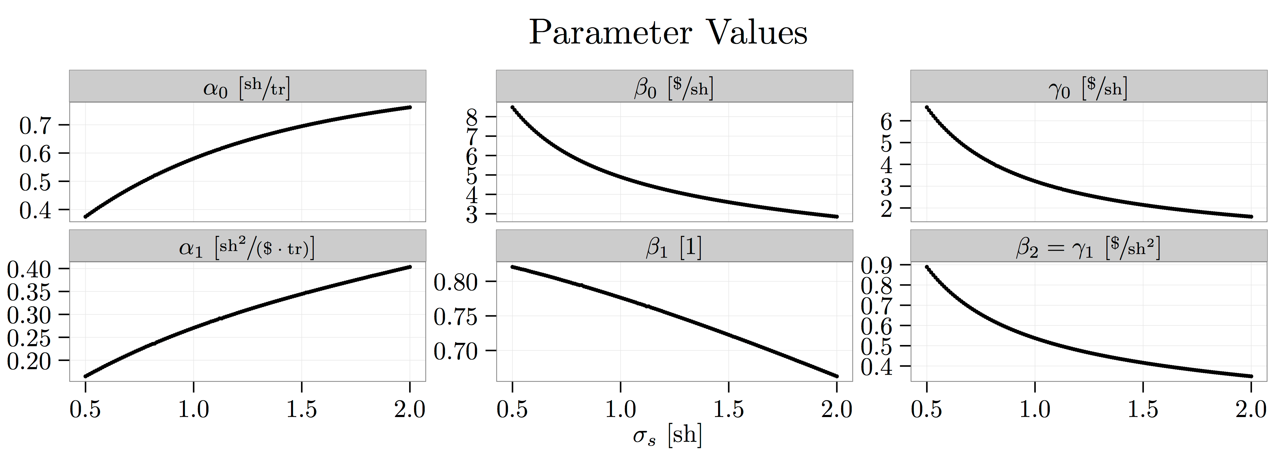
Let’s wrap up this post by looking at how the equilibrium changes as we vary the amount of noise-trader demand volatility, $\sigma_s$ . In all of the plots below, I use the following parameterization: $\sigma_v = 1$ , $\mu_s = 10$ , $\mathcal{N} = 10$ , $\phi = 1$ , and $\lambda = 1$ . You can find the code used to create these plots here.

Comparing Kyle and Grossman-Stiglitz

June 15, 2015 by Alex

1. Motivation

New information-based asset-pricing models are often extensions of either Kyle (1985) or Grossman-Stiglitz (1980). At first glance, these two canonical models look quite similar. Both price an asset with an unknown payout, like a stock or bond, and both analyze the strategic behavior of informed traders in the presence of demand noise. Yet, in spite of these similarities, the internal logic in each model is quite different.

On one hand, Kyle (1985) studies the behavior a single, large, risk-neutral, informed trader who recognizes that his own trading impacts the price. That is, he knows that, if he tries to buy more shares of the asset, then the market maker will think to herself: “Why is there more demand for this asset? Well, the informed trader probably found out some good news, so I better raise the stock price.” As a result, the informed trader buys until his expected profit from holding another share is exactly offset by the price impact of this purchase. The informed trader’s strategic behavior in Kyle (1985) is all about managing price impact.

On the other hand, Grossman-Stiglitz (1980) studies many, small, risk-averse, informed traders who take the equilibrium price as given. Rather than submitting a single request for a certain number of shares, informed traders in Grossman-Stiglitz (1980) submit a menu of price-quantity pairs that they’d be happy to buy—for example, an informed trader might be willing to buy $500$ shares at $\mathdollar 3.00$ per share, $400$ shares at $\mathdollar 3.50$ per share, $300$ shares at $\mathdollar 3.75$ per share, and so on. Informed traders choose this menu of price-quantity pairs such that, at each price level, their expected utility gain from holding another share of the stock is exactly offset by the disutility they realize from the extra variance that holding this share adds to their portfolio. Informed traders’ strategic behavior in Grossman-Stiglitz (1980) is all about managing risk.

Even though both these models end up conveying the same key idea—namely, that informed traders are more aggressive when their is more demand noise—each model arrives at this conclusion for very different reasons. So, when making modeling decisions, it’s useful to have a sense of each model’s predictions and assumptions. In this post, I work through a static version of each model with this goal in mind.

2. Kyle (1985)

Let’s start the analysis by looking at a static version of Kyle (1985). In this model, there is a single asset with an unknown payout, $\hat{v} \sim \mathrm{N}(0,\sigma_v^2)$ , where the payout is composed of two independent parts,

(1) $\begin{align*} \hat{v} &= \hat{f} + \hat{e}, \end{align*}$

with $\hat{f} \overset{\scriptscriptstyle \mathrm{iid}}{\sim} \mathrm{N}(0,\sigma_f^2)$ , $\hat{e} \overset{\scriptscriptstyle \mathrm{iid}}{\sim} \mathrm{N}(0,\sigma_e^2)$ , and $\sigma_f^2 = \lambda \cdot \sigma_v^2$ for some $\lambda \in (0,1)$ . Here, $\hat{f}$ is the knowable component of the asset’s payout, and $\hat{e}$ is the idiosyncratic component of the asset’s payout. So, for example, if $\lambda = 0.50$ , then the half of the variation in the asset’s payout can be learned and half is due to the accidents of life.

This is how trading works in Kyle (1985). An informed trader (think: arbitrageur) and a noise trader both submit market orders to a market maker—that is, the informed trader might tell the market maker, “I want to buy $500$ shares.”, and the noise trader might tell the market maker, “I want to sell $200$ shares.” While the informed trader has private information about the value of the asset and uses this information when trading, the noise trader just submits random orders, $\hat{z} \overset{\scriptscriptstyle \mathrm{iid}}{\sim} \mathrm{N}(\mu_z,\sigma_z^2)$ . The challenge facing the market maker is that she only gets to see aggregate order flow,

(2) $\begin{align*} a = x + \hat{z}. \end{align*}$

So, while she has beliefs about how likely it is that an order comes from the informed trader, she doesn’t know whether any particular order comes from the informed trader or the noise trader. To the market maker, the order flow described above just looks like, “People want to buy $300$ shares.”

Given this setup, the informed trader chooses how many shares, $x$ , to demand from the market maker,

(3) $\begin{align*} \max_{x} \, \mathrm{E}\left( \, \left( \hat{v} - p \right) \cdot x \, \middle| \, \hat{f} \, \right), \end{align*}$

knowing that, if he demands more shares, then the market maker will see this additional demand and use this information to adjust the price. The market maker tries to set the price as accurately as possible,

(4) $\begin{align*} \min_{p} \, \mathrm{E}\left( \, \left(\hat{v} - p\right)^2 \, \middle| \, a \, \right), \end{align*}$

after seeing the aggregate demand for the asset. To keep things tractable, let’s assume that both the market maker’s pricing rule, $p = \alpha + \beta \cdot a$ , and the informed trader’s demand rule, $x = \gamma + \delta \cdot \hat{f}$ , are linear. We’ll see shortly that these guesses are correct.

From here, solving the model is straightforward. First, let’s plug the functional form of the market maker’s pricing rule into the informed trader’s optimization problem:

(5) $\begin{align*} 0 = \mathrm{E}\left( \, (\hat{v} - \alpha) - 2 \cdot \beta \cdot x + \beta \cdot (\hat{z} - \mu_z) \, \middle| \, \hat{f} \, \right) &= \underbrace{\hat{f} - (\alpha + \beta \cdot x)}_{\substack{\text{Expected profit from} \\ \text{buying the $x$th share.}}} - \underbrace{\beta \cdot x}_{\substack{\text{Cost due} \\ \text{to price} \\ \text{impact of} \\ \text{$x$th share.}}}. \end{align*}$

This equation says that the informed trader will keep on trading until the expected profit that he’ll earn from buying the last share is exactly offset by the price impact of this purchase. Rearranging the terms gives a linear demand rule, $x = - \, \sfrac{\alpha}{(2 \cdot \beta)} + \sfrac{1}{(2 \cdot \beta)} \cdot \hat{f}$ , just as we guessed.

Then, let’s study to the market maker’s problem to solve for the equilibrium coefficient values. The market maker sets the price equal to her conditional expectation of the asset’s value given the aggregate demand, $\mathrm{E}( \hat{v} | a ) = \alpha + \beta \cdot a$ where $\alpha = \mathrm{E}(\hat{v}) - \beta \cdot (\mathrm{E}(x) - \mu_z)$ . But, this means that equilibrium $\beta$ is just a regression coefficient with the following functional form:

(6) $\begin{align*} \beta &= \frac{\mathrm{Cov}(\hat{v},a)}{\mathrm{Var}(a)} = \frac{1}{2} \cdot \frac{\sigma_f}{\sigma_z}. \end{align*}$

Noticing that $\delta = \sfrac{1}{(2 \cdot \beta)}$ gives the remaining coefficients:

(7) $\begin{align*} \begin{matrix} \alpha = \sqrt{\lambda} \cdot \left\{ \sfrac{\mu_z}{\sigma_z} \right\} \cdot \sigma_v, & \ & \beta = \sfrac{\sqrt{\lambda}}{2} \cdot (\sfrac{1}{\sigma_z}) \cdot \sigma_v, & \ & \gamma = - \mu_z, & \ & \text{and} & \ & \delta = \sfrac{1}{\sqrt{\lambda}} \cdot (\sfrac{1}{\sigma_v}) \cdot \sigma_z. \end{matrix} \end{align*}$

Although Kyle (1985) is no longer an accurate description of how real-world traders interact with market makers, people still use it because it’s an incredibly simple way of capturing a key fact: informed traders trade more aggressively (i.e., $\delta \nearrow$ ) when there is more noise trading (i.e., when $\sigma_z \nearrow$ ). For more detailed analysis, see my earlier posts on the 2-period Kyle (1985) model and its geometric interpretation

3. Grossman-Stiglitz (1980)

Next, let’s analyze a simplified version of Grossman-Stiglitz (1980) where there is a single asset with the same payout structure as above, $\hat{v} = \hat{f} + \hat{e}$ . In this model, there are now many informed traders take the equilibrium price as given and solve the optimization problem below,

(8) $\begin{align*} \max_x \, \mathrm{E}\left( \, - e^{- \phi \cdot w} \, \middle| \, \hat{f}, \, p \, \right) \quad \text{subject to} \quad w = \bar{w} + (\hat{v} - p) \cdot x, \end{align*}$

where $\phi$ is the informed traders’ risk-aversion parameter in units of $\sfrac{1}{\mathdollar}$ . Note that this means the traders are now trying to maximize utility rather than profits. Solving this problem, we see that

(9) $\begin{align*} 0 &= \underbrace{\hat{f} - p}_{\substack{\text{Expected utils} \\ \text{gained from} \\ \text{buying $x$th} \\ \text{share at} \\ \text{price $p$.}}} - \underbrace{\phi \cdot \sigma_e^2 \cdot x}_{\substack{\text{Utils lost due} \\ \text{to increased risk} \\ \text{from buying $x$th} \\ \text{share at price $p$.}}}. \end{align*}$

That is, at each price level, the informed traders trade until their expected utility gain from holding another share of the risky asset is exactly offset by the disutility they realize from the extra variance that holding this share adds to their portfolio. Rearranging this expression then gives their optimal portfolio position at each price level, $x = (\phi \cdot \sigma_e)^{-1} \times \{\sfrac{(\hat{f} - p)}{\sigma_e}\}$ . So, informed traders buy shares whenever the equilibrium price is below their signal about the asset’s expected value, and they buy relatively more shares when they are less risk averse and when their information is more precise.

There is no explicit market maker learning from aggregate order flow in Grossman-Stiglitz (1980) like there is in Kyle (1980); instead, there is a collection of uninformed traders who observe the equilibrium price of the asset, $p$ , and use this information to guide their trading. Each of these uninformed traders solves the same optimization problem as the informed traders,

(10) $\begin{align*} \max_y \, \mathrm{E}\left( \, - e^{- \varphi \cdot w} \, \middle| \, p \, \right) \quad \text{subject to} \quad w = \bar{w} + (\hat{v} - p) \cdot y, \end{align*}$

where $\varphi$ is the informed traders’ risk-aversion parameter in units of $\sfrac{1}{\mathdollar}$ . Solving this problem, we see that

(11) $\begin{align*} 0 &= \underbrace{\mathrm{E}(\hat{f}|p) - p}_{\substack{\text{Expected utils} \\ \text{gained from} \\ \text{buying $y$th} \\ \text{share at price $p$.}}} - \underbrace{\varphi \cdot (\mathrm{Var}(\hat{f}|p) + \sigma_e^2) \cdot y}_{\substack{\text{Utils lost due} \\ \text{to increased risk} \\ \text{from buying $y$th} \\ \text{share at price $p$.}}}. \end{align*}$

That is, at each price level, the uninformed traders trade until their expected utility gain from holding another share of the risky asset is exactly offset by the disutility they realize from the extra variance that holding this share adds to their portfolio. This is exactly the same demand rule that the informed traders use. The only difference is that they don’t have a private signal, $\hat{f}$ , about the asset’s fundamental value. Just like before, rearranging this expression then gives the uninformed traders’ optimal portfolio position at each price level, $y = \varphi^{-1} \cdot \mathrm{StD}(\hat{v}|p)^{-1} \times \{ \sfrac{(\mathrm{E}(\hat{f}|p) - p)}{\mathrm{StD}(\hat{v}|p)}\}$ .

Yet, there is something slightly puzzling about the setup of the Grossman-Stiglitz (1980) model so far. What does it mean for traders to condition on the price? How can they already know this? The short answer is: they don’t. Rather than submitting market orders like in Kyle (1980), traders in Grossman-Stiglitz (1980) submit a menu of price-quantity pairs that they’d be happy trading and then the equilibrium price is pinned down by a menu auction. If there was some uncertainty as to how many shares of the asset were available due to noise trader demand and all traders (both informed and uninformed) submitted a menu of price-quantity pairs,

(12) $\begin{align*} \hat{z} &= \int x_i \cdot di + \int y_u \cdot du \end{align*}$

then the market-clearing price and demand that would be chosen by an auctioneer is the same as the Grossman-Stiglitz (1980) price and demand.

This auction-like equilibrium concept means that informed traders are solving a fundamentally different problem in Grossman-Stiglitz (1980). In Grossman-Stiglitz (1980), the informed traders don’t know how many shares of the risky asset they will end up buying and have to optimally choose an entire menu of price-quantity pairs. In Kyle (1980), by contrast, the informed trader knows exactly how many shares of the risky asset he will buy, he just doesn’t know what the resulting price will be. He solving a much simpler problem in Kyle (1980) since he only has to optimally pick a single number rather than an entire menu.

Once we’ve setup the model, solving it is again relatively straightforward. Just like in Kyle (1980), let’s guess that the equilibrium pricing rule is linear, $p = \eta + \theta \cdot \hat{f} - \beta \cdot \hat{z}$ , where $\eta$ has units of $\sfrac{\mathdollar}{\text{share}}$ , $\theta$ is dimensionless, and $\beta$ has units of $\sfrac{\mathdollar}{\text{shares}^2}$ . Thus, if the uninformed traders only condition on the price of the risky asset when making their portfolio choice, they will have the following signal about $\hat{f}$ :

(13) $\begin{align*} \frac{p - (\eta - \beta \cdot \mu_z)}{\theta} &= \hat{f} - \frac{\beta}{\theta} \cdot (\hat{z} - \mu_z). \end{align*}$

This means that they will have beliefs,

(14) $\begin{align*} \mathrm{Var}(\hat{f}|p) &= \left\{ \frac{\beta^2 \cdot \sigma_z^2}{\beta^2 \cdot \sigma_z^2 + \theta^2 \cdot \sigma_f^2} \right\} \times \sigma_f^2 \\ \mathrm{E}(\hat{f}|p) &= \left\{ \frac{\theta^2 \cdot \sigma_f^2}{\beta^2 \cdot \sigma_z^2 + \theta^2 \cdot \sigma_f^2} \right\} \times \frac{p - (\eta - \beta \cdot \mu_z)}{\theta}. \end{align*}$

To simplify the notation below, let’s define a new dimensionless constant, $\kappa = \sfrac{(\theta^2 \cdot \sigma_f^2)}{(\beta^2 \cdot \sigma_z^2 + \theta^2 \cdot \sigma_f^2)}$ , which represents how much weight the uninformed traders put on the price signal. When $\kappa \approx 1$ , uninformed traders learn a lot from the price; whereas, when $\kappa \approx 0$ , uninformed traders learn very little from the price.

To solve for the coefficients $\eta$ , $\theta$ , and $\beta$ we then need to enforce the market-clearing condition,

(15) $\begin{align*} \hat{z} &= \int_0^{\sfrac{1}{2}} x_i \cdot di + \int_{\sfrac{1}{2}}^1 y_u \cdot du, \end{align*}$

where I’m assuming for simplicity that half of the traders are informed and half are uninformed. Allowing traders to optimally choose their information like in the original Grossman-Stiglitz (1980) model doesn’t change the basic comparison to the Kyle (1980) setup and complicates the analysis. If we substitute the functional forms for traders’ demand into the market-clearing condition, then we get:

(16) $\begin{align*} 2 \cdot \varphi \cdot \hat{z} &= \frac{\varphi}{\phi} \cdot \left( \frac{\hat{f} - p}{\sigma_e^2} \right) + \left( \frac{\mathrm{E}(\hat{f}|p) - p}{\mathrm{Var}(\hat{f}|p) + \sigma_e^2} \right). \end{align*}$

Rearranging this expression then gives us an expression for the equilibrium price that is linear in the price signal, $\hat{f}$ , and then noise trader demand, $\hat{z}$ ,

(17) $\begin{align*} p &= - \, \{ \xi^{-1} \cdot (1 - \lambda) \cdot (\sfrac{\kappa}{\theta}) \} \cdot (\eta - \beta \cdot \mu_z) \\ &\qquad + \, \{ \xi^{-1} \cdot (\sfrac{\varphi}{\phi}) \cdot (1 - \kappa \cdot \lambda) \} \cdot \hat{f} \\ &\qquad \qquad - \, 2 \cdot \{\xi^{-1} \cdot (1 - \lambda) \cdot (1 - \kappa \cdot \lambda)\} \cdot \varphi \cdot \sigma_v^2 \cdot \hat{z}, \end{align*}$

with $\xi = (\sfrac{\varphi}{\phi}) \cdot (1 - \kappa \cdot \lambda) - \sfrac{(\kappa - \theta)}{\theta} \cdot (1 - \lambda)$ . Matching the coefficients and solving then yields the equilibrium values

(18) $\begin{align*} \begin{matrix} \eta = \left\{ \frac{\kappa \cdot (1 - \lambda)}{\xi \cdot \theta + \kappa \cdot (1 - \lambda)} \right\} \cdot \beta \cdot \mu_z, & & \theta = \xi^{-1} \cdot (\sfrac{\varphi}{\phi}) \cdot (1 - \kappa \cdot \lambda), & \ \text{and} \ & \beta = 2 \cdot \{\theta \cdot (1 - \lambda)\} \cdot \phi \cdot \sigma_v^2. \end{matrix} \end{align*}$

4. Comparative Statics

Now that we’ve seen how each model works, let’s look at some comparative statics to better understand how each model’s predictions differ. Unless stated otherwise, I use the following parameter values in the plots below: $\sigma_v = \sfrac{\mathdollar 1}{\text{sh}}$ , $\mu_z = 1{\scriptstyle \mathrm{sh}}$ , $\sigma_z = 1{\scriptstyle \mathrm{sh}}$ , $\lambda = \sfrac{1}{2}$ , $\phi = \sfrac{1}{\mathdollar}$ , and $\varphi = \sfrac{1}{\mathdollar}$ . For each outcome variable, I look at how the predictions of each model as I vary the quality of the informed traders’ information, $\lambda$ , from $0 \to 1$ , the level of the informed traders’ risk aversion, $\phi$ , from $0 \to 2$ , and the volatility of noise traders’ demand, $\sigma_z$ , from $0 \to 2$ . If you’d like to look at other parameterizations, you can find all of the code here.

Let’s begin by looking at informed traders’ demand response in each model. That is, if the informed traders’ private signal about the value of risky asset increases by $\mathdollar 1$ per share, then how many additional shares will the informed trader typically demand? In the Kyle (1980), this is just the equilibrium $\beta$ :

(19) $\begin{align*} \mathrm{E}\left( \frac{\partial x}{\partial \hat{f}} \right) &= \beta = \frac{1}{\sqrt{\lambda}} \cdot \frac{1}{\sigma_v} \cdot \sigma_z. \end{align*}$

By contrast, this expression takes on a more complicated functional form in Grossman-Stiglitz (1980):

(20) $\begin{align*} \mathrm{E}\left( \frac{\partial x}{\partial \hat{f}} \right) &= \frac{1}{\phi} \cdot \frac{1}{\sigma_v^2} \cdot \left\{ \frac{1 - \theta}{1 - \lambda} \right\}. \end{align*}$

The left-most panel of the figure below shows that, as the quality of the informed traders’ private signal increases, they they trade less aggressively in both models. That is, informed traders demand fewer additional shares of the risky asset per $\mathdollar 1$ increase in the private signal, $\hat{f}$ .

Similarly, the right-most panel of the figure shows that, as the noise-trader-demand volatility increases, informed traders trade more aggressively in both models. It’s important to note, however, that this effect is driven by very different forces in each model. In Kyle (1980), the informed trader trades more aggressively when there is more demand noise because the additional noise lowers his price impact. By comtrast, in Grossman-Stiglitz (1980) informed traders trade more aggressively when there is more demand noise because this additional noise makes the equilibrium price signal less informative for the uninformed traders.

In addition to informed traders’ demand responses, there are lots of other statistics of interest. For instance, how does the average price vary with the amount of noise trading? In Kyle (1980), the answer is simple: it doesn’t. In fact, the expected price of the asset is always equal to its expected value:

(21) $\begin{align*} \mathrm{E}(p) &= \alpha - \beta \cdot (\gamma - \mu_z) = 0. \end{align*}$

In Grossman-Stiglitz (1980), however, the average price of the asset,

(22) $\begin{align*} \mathrm{E}(p) &= \eta - \beta \cdot \mu_z, \end{align*}$

can vary quite a bit with the level of noise-trader-demand volatility as shown in the right-most panel of the figure below. This risk premium comes from the fact that, if there is more noise-trader-demand volatility, then the risk-averse traders have to bear more risk, so they will be willing to pay less for the asset.

Finally, let’s take a look at the equilibrium price response, $\mathrm{E}(\sfrac{\partial p}{\partial\! \hat{f}})$ , in each model. That is, on average, how much higher is the price when the informed traders’ private signal is $\mathdollar 1$ per share higher? For the Kyle (1980) model, the answer is always:

(23) $\begin{align*} \sfrac{1}{2} = \beta \cdot \delta. \end{align*}$

In the Grossman-Stiglitz (1980) model, the answer corresponds to the equilibrium $\theta$ parameter. We see in the right-most panel of the figure below that, if there is more noise-trader-demand volatility, then the equilibrium price in the Grossman-Stiglitz (1980) model becomes less informative. Note that there is absolutely no effect in the Kyle (1980) model, where the informed trader strategically dials up the aggressiveness of his demand rule whenever noise-trader-demand volatility increases to ensure that $\sfrac{1}{2} = \beta \cdot \delta$ . So, if you want to make predictions linking the information content of prices to noise-trader-demand volatility, you’d better use Grossman-Stiglitz (1980).

5. Fine Tuning

Let me conclude by making one last observation about trying to reverse engineer the models to line up more precisely. The middle panel of each of the 3 figures above shows how the predictions of the Kyle (1980) and Grossman-Stiglitz (1980) models change as I increase informed traders’ risk aversion parameter. In every one of these panels, the predictions of the Kyle (1980) model are always flat. They have to be. The informed trader in Kyle (1980) is risk-neutral, so varying this parameter can’t have any affect of the model’s predictions. Is there any way to tune this parameter to get the models to line up more precisely?

Yes and no. No in the sense that, if you look at the middle panels in the average price and price response plots, you can see that increasing the informed traders’ risk aversion has different effects on these two outcomes, so you can’t get the two models to agree on both of these predictions by monkeying around with one tuning parameter. You’d need to fine tune the risk-aversion parameters of both the informed and the uninformed traders to do this. So it is possible if you really want to.

Even when the models give qualitatively similar predictions, like for informed traders’ demand responses, fine tuning informed traders’ risk-aversion parameter to get the models to agree quantitatively means making really strong assumptions about other parameters of the model. Specifically, notice that the demand response in Grossman-Stiglitz (1980) is identical to the demand response in Kyle (1980) if the informed traders’ risk-aversion parameter is precisely:

(24) $\begin{align*} \phi &= \left\{ \frac{\sqrt{\lambda}}{1 - \lambda} \right\} \cdot \frac{1 - \theta}{\sigma_v \cdot \sigma_z}. \end{align*}$

But, this means that deep parameters like the asset’s payout volatility, $\sigma_v$ , and the volatility of noise-trader demand, $\sigma_z$ , can only occur in certain pairs. For instance, the plot below shows the permissible values when $\lambda = \sfrac{1}{2}$ and $\varphi = \sfrac{1}{\mathdollar}$ . We see that, in order to make Kyle (1980) and Grossman-Stiglitz (1980) give quantitatively similar predictions about informed traders’ demand responses, payout volatility and noise-trader-demand volatility have to be inversely related and often orders of magnitude apart.

Comparing “Explanations” for the iVol Puzzle

May 5, 2015 by Alex

1. Motivation

A stock’s idiosyncratic-return volatility is the root-mean-squared error, $\mathit{ivol}_{n,t} = \sqrt{ \sfrac{1}{D_t} \cdot \sum_{d_t=1}^{D_t} \varepsilon_{n,d_t}^2}$ , from the daily regression

(1) $\begin{align*} r_{n,d_t} = \alpha + \beta_{\mathit{Mkt}} \cdot r_{\mathit{Mkt},d_t} + \beta_{\mathit{SmB}} \cdot r_{\mathit{SmB},d_t} + \beta_{\mathit{HmL}} \cdot r_{\mathit{HmL},d_t} + \varepsilon_{n,d_t}. \end{align*}$

Ang, Hodrick, Xing, and Zhang (2006) shows that stocks with lots of idiosyncratic-return volatility in the previous month have extremely low returns in the current month. To quantify just how low these returns are, I run a cross-sectional regression each month,

(2) $\begin{align*} r_{n,t} &= \mu_{r,t} + \beta_t \cdot \widetilde{\mathit{ivol}}_{n,t-1} + \epsilon_{n,t} \end{align*}$

where $\widetilde{\mathit{ivol}}_{n,t} = \sfrac{(\mathit{ivol}_{n,t} - \mu_{\mathit{ivol},t})}{\sigma_{\mathit{ivol},t}}$ . Over the period from January 1965 to December 2012, I estimate that a trading strategy which is long the stocks with higher-than-average idiosyncratic-return volatility in the previous month and short the stocks with lower-than-average idiosyncratic-return volatility in the previous month,

(3) $\begin{align*} \beta_t &= \frac{1}{N \cdot \sigma_{\mathit{ivol},t-1}} \cdot \sum_n \left( \mathit{ivol}_{n,t-1} - \mu_{\mathit{ivol},t-1} \right) \cdot r_{n,t}, \end{align*}$

has an average excess returns of $\langle \beta_t \rangle = -0.98{\scriptstyle \%}$ per month or $-10.05{\scriptstyle \%}$ per year.

This is puzzling on two levels. First, standard asset-pricing theory says that traders shouldn’t be compensated for holding diversifiable risk, so it’s surprising that idiosyncratic-return volatility is priced at all. “But, wait a second.”, you say. “Maybe there’s some friction that makes it hard to diversify-away some of this idiosyncratic risk.” Right. Here’s where the second level comes in. If this were the case, if what we’re calling idiosyncratic-return volatility was somehow non-diversifiable, then you’d expect stocks with lots of idiosyncratic-return volatility to trade at a discount, not a premium. You’d expect these stocks to earn higher returns to compensate traders for holding additional risk, not lower returns. The results in Ang, Hodrick, Xing, and Zhang (2006) are so interesting because they suggest that idosyncratic-return volatility is not only priced but priced wrong. People don’t just care about idiosyncratic-return volatility, they covet it.

Since 2006 there have been numerous papers that have attempted to explain this puzzling result. But, how can we tell if an explanation is good? In this post, I show how to answer this question using techniques introduced in Hou and Loh (2014). You can find all the code here. The data comes from WRDS.

2. Standard Approach

The standard approach for testing to see if a candidate variable explains the idiosyncratic-return-volatility puzzle involves two stages. In the first stage, people show that the candidate variable is a strong predictor of idiosyncratic-return volatility in a cross-sectional regression,

(4) $\begin{align*} \widetilde{\mathit{ivol}}_{n,t} &= \gamma_t \cdot \widetilde{x}_{n,t} + \xi_{n,t}, \end{align*}$

where $\widetilde{x}_{n,t} = \sfrac{(x_{n,t} - \mu_{x,t})}{\sigma_{x,t}}$ . So, for example, if the candidate variable is the maximum daily return in the previous month as suggested in Bali, Cakici, and Whitelaw (2011), then this first-stage regression verifies that the stocks with the highest maximum return in any given month also have the most idiosyncratic-return volatility.

In the second stage, people then run a horse-race regression to see if the candidate variable “drives out” the significance of idiosyncratic-return volatility when predicting monthly returns:

(5) $\begin{align*} r_{n,t} &= \mu_{r,t} + \beta_t \cdot \widetilde{\mathit{ivol}}_{n,t-1} + \delta_t \cdot \widetilde{x}_{n,t-1} + \epsilon_{n,t}. \end{align*}$

The idea behind this second-stage regression is simple. If the estimated $\langle \beta_t \rangle = 0$ and $\langle \delta_t \rangle < 0$ , then the candidate variable explains both a) which stocks had lots of idiosyncratic-return volatility in the the previous month and b) which stocks realized very low returns in the current month.

But, what happens if $\langle \beta_t \rangle < 0$ and $\langle \delta_t \rangle < 0$ , meaning that the candidate variable doesn’t explain all of the idiosyncratic-return-volatility puzzle? How can we tell how much of the idiosyncratic-return-volatility puzzle is explained by a given candidate? This two-stage regression procedure can’t answer this question.

3. Alternative Strategy

To understand how much of the puzzle is explained by, say, a stock’s maximum daily return in the previous month, we need to decompose the excess returns to trading on idiosyncratic-return volatility into two components, namely, the part explained by a stock’s maximum return and everything else:

(6) $\begin{align*} \beta &= \mathrm{Cov}[ \, r_{n,t} , \, \widetilde{\mathit{ivol}}_{n,t-1} \, ] \\ &= \mathrm{Cov}\left[ \, r_{n,t}, \, \gamma_t \cdot \widetilde{x}_{n,t-1} + \xi_{n,t-1} \, \right] \\ &= \underbrace{\gamma_t \cdot \mathrm{Cov}\left[ \, r_{n,t}, \, \widetilde{x}_{n,t-1} \, \right]}_{\text{Explained}} + \underbrace{\mathrm{Cov}\left[ \, r_{n,t}, \, \xi_{n,t-1} \, \right]}_{\substack{\text{Everything} \\ \text{Else}}} \end{align*}$

This explained part is just the returns to a trading strategy that is long the stocks with a higher-than-average value of the candidate variable in the previous month and short the stocks with a lower-than-average value of the candidate variable in the previous month,

(7) $\begin{align*} \beta_{E,t} &= \gamma_t \cdot \mathrm{Cov}\left[ \, r_{n,t}, \, \widetilde{x}_{n,t-1} \, \right] = \frac{\gamma_t}{N \cdot \sigma_{x,t-1}} \cdot \sum_n \left( x_{n,t-1} - \mu_{x,t-1} \right) \cdot r_{n,t}, \end{align*}$

with the portfolio position scaled by the predictive power of the candidate variable over idiosyncratic-return volatility, $\gamma_t$ . Put differently, a candidate variable explains a lot of the idiosyncratic-return-volatility puzzle if it is a good predictor of idiosyncratic-return volatility, $\gamma_t > 0$ , and it generates negative returns when you trade on it, $(N \cdot \sigma_{x,t-1})^{-1} \cdot \sum_n( x_{n,t-1} - \mu_{x,t-1}) \cdot r_{n,t} < 0$ .

If we have an expression for the explained component of the idiosyncratic-return-volatility puzzle, then we can use GMM to estimate it. Let $\mathbf{\Theta}_t$ be a vector of coefficients to be estimated in month $t$ ,

(8) $\begin{align*} \mathbf{\Theta}_t &= \begin{bmatrix} \mu_{r,t} & \beta_t & \gamma_t & \beta_{E,t} \end{bmatrix}, \end{align*}$

using the cross-section of all NYSE, AMEX, and NASDAQ stocks in the WRDS. We can then estimate this $(1 \times 4)$ -dimensional vector of coefficients using the following moment conditions:

(9) $\begin{align*} g_N(\mathbf{\Theta}_t) &= \frac{1}{N} \cdot \sum_n \begin{pmatrix} r_{n,t} - \mu_{r,t} - \beta_t \cdot \widetilde{\mathit{ivol}}_{n,t-1} \\ \left( r_{n,t} - \mu_{r,t} - \beta_t \cdot \widetilde{\mathit{ivol}}_{n,t-1} \right) \cdot \widetilde{\mathit{ivol}}_{n,t-1} \\ \left( \widetilde{\mathit{ivol}}_{n,t-1} - \gamma_t \cdot \widetilde{x}_{n,t-1} \right) \cdot \widetilde{x}_{n,t-1} \\ \beta_{E,t} - \gamma_t \cdot r_{n,t} \cdot \widetilde{x}_{n,t-1} \end{pmatrix}, \end{align*}$

where the first two moments estimate the OLS regression in Equation (2), the third moment estimates the OLS regression in Equation (4), and the fourth moment estimates the explained component of the idiosyncratic-return-volatility puzzle as given in Equation (7). When I estimate these $4$ coefficients each month for the maximum return candidate explanation, I find that the explained return is $-0.84{\scriptstyle \%}$ per month, or about $\sfrac{0.84}{0.99} = 85{\scriptstyle \%}$ of the total puzzle.

$plot--ivol-puzzle--fraction-explained$

4. What Counts As An “Explanation”?

One of the nice things about setting up the problem up this way—as opposed to using approximation methods like in the original Hou and Loh (2014) article—is that it makes really clear what an explanation is. A candidate variable is a good explanation of the idiosyncratic-return-volatility puzzle if you can’t make (or lose) money by trading on idiosyncratic-return volatility that isn’t predicted by the candidate variable:

(10) $\begin{align*} \text{``Everything Else'' term in Equation (6)} &= \frac{1}{N} \cdot \sum_n \left( \widetilde{\mathit{ivol}}_{n,t-1} - \gamma_t \cdot \widetilde{x}_{n,t-1} \right) \cdot r_{n,t}. \end{align*}$

Note that this is a very particular definition of “explained”. Usually, when you think about an explanation, you have in mind some causal mechanism. But, that’s not what’s meant here. It’s not as if you could give some stocks higher idiosyncratic-return volatility and lower future returns by randomly assigning them higher maximum returns in the current month and not changing any of their other properties. Clearly, there is some deeper mechanism as play that’s causing both higher idiosyncratic-return volatility and higher maximum returns. But, you can’t trade on the part of idiosyncratic-return volatility that’s not explained by the maximum return.

« Previous Page