1. Introduction
In my paper Feature Selection Risk (2014), I study a problem where assets have  different attributes and traders try to identify which
  of these attributes matter via price changes:
(1) ![\begin{align*} \Delta p_n &= p_n - \mathrm{E}[p_n] = \sum_{q=1}^Q \beta_q \cdot x_{n,q} + \epsilon_n \qquad \text{where} \qquad K = \Vert {\boldsymbol \beta} \Vert_{\ell_0} = \sum_{q=1}^Q 1_{\{ \beta_q \neq 0 \}} \notag \end{align*}](https://alexchinco.com/wp-content/ql-cache/quicklatex.com-61b486123cee5de4e870b72d62eeaa04_l3.svg "Rendered by QuickLaTeX.com")
with each asset’s exposure to a given attribute given by  and the noise is given by
  . In the limit as
  ,
,  ,
,  , and
, and  there exists both a signal opacity bound,
  , as well as a signal recovery bound,
  :
:
(2) 
with  in units of transactions. I explain what I mean by “
 ” in Section 4 below. These
  thresholds separate the regions where traders are arbitrarily bad at identifying the shocked attributes (i.e.,
  ) from the regions where traders can almost surely identify the shocked attributes (i.e.,
  ). i.e., if traders have seen fewer than transactions, then they have no idea which shocks took place; whereas, if traders have seen more than transactions, then they can pinpoint exactly which shocks took place.
In this post, I show that the signal opacity and recovery bounds become arbitrarily close in a large market. The analysis in this post primarily builds on work done in Donoho and Tanner (2009) and Wainwright (2009).
2. Motivating Example
This sort of inference problem pops up all the time in financial settings. Suppose you moved away from Chicago a year ago, and now you’re moving back and looking for a house. When studying a list of recent sales prices, you find yourself a bit surprised. People seem to have changed their preferences for  of
of  different amenities:
  a car garage,
  a third bedroom,
  a half-circle driveway,
  granite countertops,
  energy efficient appliances,
  central A/C, or
  a walk-in closet? The mystery amenity is raising the sale price of some houses by
  dollars. How many sales do you need to see in order to figure out which of the amenities realized the shock?
The answer is  . How did I arrive at this number? Suppose you found one house with amenities
  , a second house with amenities
  , and a third house with amenities
  . The combination of the price changes for these houses reveals exactly which amenity has been shocked. i.e., if only the first house’s price was too high,
 ![\Delta p_1 = p_1 - \mathrm{E}[p_1] = \beta](https://alexchinco.com/wp-content/ql-cache/quicklatex.com-192f208edef697e5db9b60ed0bf7e90d_l3.svg "Rendered by QuickLaTeX.com") , then Chicagoans must have changed their preferences for car garages:
, then Chicagoans must have changed their preferences for car garages:
(3) 
By contrast, if  , then people must value walk-in closets more than they did a year ago.
Here’s the key point. The problem changes character at  observations. sales is just enough information to answer yes or no questions and rule out the possibility of no change:
  .
.  sales simply narrows your error bars around the exact value of
  .
.  sales only allows you to distinguish between subsets of amenities. e.g., seeing just the first and second houses with unexpectedly high prices only tells you that people like either half-circle driveways or walk-in closets more… not which one.
Yet, the dimensionality in this toy example can be confusing. There is obviously something different about the problem at observations, but there is still some information contained in the first observations. e.g., even though you can’t tell exactly which attribute realized a shock, you can narrow down the list of possibilities to attributes out of . If you just flipped a coin and guessed after seeing transactions, you would have an error rate of  . This is no longer true in higher dimensions. i.e., even in the absence of any noise, seeing any fraction
  of the required observations for
  will leave you with an error rate that is within a tiny neighborhood of
  as the number of attributes gets large.
3. Non-Random Analysis
I start by exploring how the required number of observations, , moves around as I increase the number of attributes in the setting where there is only  shock and the data matrix is non-random. Specifically, I look at the case where and
  . My goal is to build some intuition about what I should expect in the more complicated setting where the data
  is a random matrix. Here, in this simple setting, the ideal data matrix would be
  -dimensional and look like:
(4) ![\begin{equation*} \underset{4 \times 15}{\mathbf{X}} = \left[ \begin{matrix} 1 & 0 & 1 & 0 & 1 & 0 & 1 \\ 0 & 1 & 1 & 0 & 0 & 1 & 1 \\ 0 & 0 & 0 & 1 & 1 & 1 & 1 \\ 0 & 0 & 0 & 0 & 0 & 0 & 0 \end{matrix} \ \ \ \begin{matrix} 0 & 1 & 0 & 1 & 0 & 1 & 0 & 1 \\ 0 & 0 & 1 & 1 & 0 & 0 & 1 & 1 \\ 0 & 0 & 0 & 0 & 1 & 1 & 1 & 1 \\ 1 & 1 & 1 & 1 & 1 & 1 & 1 & 1 \end{matrix} \right] \end{equation*}](https://alexchinco.com/wp-content/ql-cache/quicklatex.com-c9654d5e3c73000da35573acd23905a3_l3.svg "Rendered by QuickLaTeX.com")
where each column of the data matrix corresponds to a number  in binary.
Let  be a function that eats
  observed price changes and spits out the set of possible preference changes that might explain the observed price changes. e.g., if traders only see the st transaction, then they can only place the shock in of sets containing
  attributes each:
(5) 
The nd transaction then allows traders to split each of these larger sets into smaller ones and place the shock in a set of  possibilities:
(6) 
With the rd transaction, traders can tell that the actual shock is either of possibilities:
(7) 
The  th observation then closes the case against the offending attribute.
Here’s the key observation. Only the absolute difference between  matters when computing the size of the output of . If traders have seen
  transaction, then they can tell which subset of
  attributes has realized a shock. If traders have seen
  transactions, then they can tell which subset of
  attributes has realized a shock. If traders have seen
  observations, then they can tell which subset of
  attributes has realized a shock. Thus, after seeing any number of observations
  , traders can place the shock in a set of size
  . i.e., a trader has the same amount of information about which attribute has realized a shock in (i) a situation where
  and he’s seen
  transactions as in (ii) a situation where and he’s seen transactions.
The probability that traders select the correct attribute after seeing only observations is given by  assuming uniform priors. Natural numbers are hard to work with analytically, so let’s suppose that traders observe some fraction of the required number of observations . i.e., for some traders see
  observations. We can then perform a change of variables
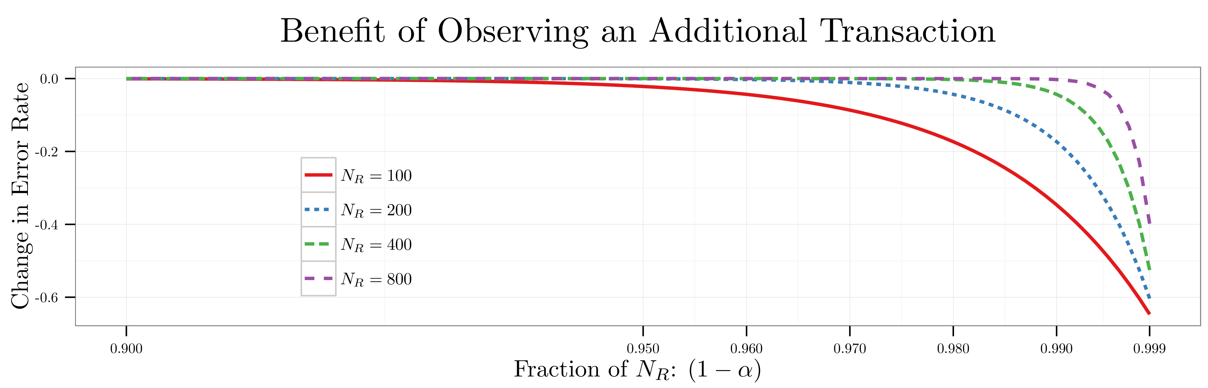
  and answer the question: “How much does getting additional observation improve traders’ error rate?”
(8) ![\begin{align*} \frac{1}{N_R} \cdot \frac{d}{d\alpha}\left[ \, 2^{- (N_R - N)} \, \right] = - \log(2) \cdot e^{- \alpha \cdot \log(2) \cdot N_R} \end{align*}](https://alexchinco.com/wp-content/ql-cache/quicklatex.com-aed714b93d9cbbf093a71edae530f1c7_l3.svg "Rendered by QuickLaTeX.com")
I plot this statistic for ranging from  to
to  below. When , a trader’s predictive power doesn’t start to improve until he sees
  transactions (i.e.,
  of ); by contrast, when
  a trader’s predictive power doesn’t start to improve until he’s seen
  transactions (i.e.,
  of ). Here’s the punchline. As I scale up the original toy example from attributes to million attributes, traders effectively get
  useful information about which attributes realized a shock until they come within a hair’s breadth of the signal recovery bound . The opacity and recovery bounds are right on top of one another.
4. Introducing Randomness
Previously, the matrix of attributes was strategically chosen so that the set of observations that traders see would be as informative as possible. Now, I want to relax this assumption and allow the data matrix to be random with elements  :
:
(9) 
where  denotes idiosyncratic shocks affecting asset
  in units of dollars. For a given triplet of integers
  with
with  , I want to know whether solving the linear program:
(10) 
recovers the true  when it is
  -sparse. i.e., when has only non-zero entries
  . Since
  the linear system is underdetermined; however, if the level of sparsity is sufficiently high (i.e., is sufficiently small), then there will be a unique solution with high probability.
First, I study the case where there is no noise (i.e., where  ), and I ask: “What is the minimum number of observations needed to identify the true with probability
  for
for  using the linear program in Equation (10)?” I remove the noise to make the inference problem as easy as possible for traders. Thus, the proposition below which characterizes this minimum number of observations gives a lower bound. I refer to this number of observations as the signal opacity bound and write it as . The proposition shows that, whenever traders have seen observations, I can make traders’ error rate arbitrarily bad (i.e.,
  ) by increasing the number of attributes (i.e.,
  ).
).
Proposition (Donoho and Tanner, 2009): Suppose  ,
,  , and
, and  with
with  . The linear program in Equation (10) will recover a fraction if the time whenever:
(11) 
where  .
.
Next, I turn to the case where there is noise (i.e., where  ), and I ask: “How many observations do traders need to see in order to identify the true with probability in an asymptotically large market using the linear program in Equation (10)?” Define traders’ error rate after seeing observations as:
(12) ![\begin{align*} \mathrm{Err}[N] &= \frac{1}{{Q \choose K}} \cdot \sum_{\substack{\mathcal{K} \in \mathcal{Q} \\ |\mathcal{K}| = K}} \mathrm{Pr}(\widehat{\boldsymbol \beta} \neq {\boldsymbol \beta}) \end{align*}](https://alexchinco.com/wp-content/ql-cache/quicklatex.com-34cf0d5b92083a52a184ce78eec484c8_l3.svg "Rendered by QuickLaTeX.com")
 denotes the probability that the linear program in Equation (10) chooses the wrong subset of attributes (i.e., makes an error) given the true support
  and averaging over not only the measurement noise,
  , but also the choice of the Gaussian attribute exposure matrix, . Traders’ error rate is the weighted average of these probabilities over every shock set of size . Traders identify the true
  with probability in an asymptotically large market if:
(13) ![\begin{align*} \lim_{\substack{K,N,Q \to \infty \\ \sfrac{K}{Q} \to 0}} \mathrm{Err}[N] &= 0 \end{align*}](https://alexchinco.com/wp-content/ql-cache/quicklatex.com-58c9bb88049ae8e5206718106055daf5_l3.svg "Rendered by QuickLaTeX.com")
Thus, the proposition below which characterizes this number of observations gives an upper bound of sorts. I refer to this number of observations as the signal recovery bound and write it as . i.e., the proposition shows that, whenever traders have seen observations, they will be able to recovery almost surely no matter how large I make the market.
Proposition (Wainwright, 2009): Suppose , , , and , then traders can identify the true with probability in an asymptotically large market if for some constant  :
:
(14) 
The only cognitive constraint that traders face is that their selection rule must be computationally tractable. Under minimal assumptions a convex optimization program is computationally tractable in the sense that the computational effort required to solve the problem to a given accuracy grows moderately with the dimensions of the problem. Natarajan (1995) explicitly shows that  constrained linear programming is NP-hard. This cognitive constraint is really weak in the sense that any selection rule that you might look up in an econometrics or statistics textbook (e.g., forward stepwise regression or LASSO) is going to be computationally tractable. After all, they have to be executed on computers.
5. Discussion

What is really interesting is that the signal opacity bound, , and the signal recovery bound, , basically sit right on top of one another when the market gets large just as you would expect from the analysis in Section 3. The figure above plots each bound on a log-log scale for varying levels of sparsity. It’s clear from the figure that the bounds are quite close. The figure below plots the relative gap between these bounds:
(15) 
i.e., it plots how big the gap is relative to the size of the signal recover bound . For each level of sparsity, the gap is shrinking as I add more and more attributes. This is an identical result as in the figure from Section 3: as the size of the market increases, traders learn next to nothing from each successive observation until they get within an inch of the signal recovery bound. The only difference here is that now there are an arbitrary number of shocks and the data matrix is random.

 or
or  . i.e., I exclude things like ADRs, closed-end funds, and REITS. I calculate weekly returns by compounding daily returns between adjacent Wednesdays:
 industry classification system from
  different GICS industry subgroups.
 to denote the number of securities in industry
  in year
  . In each of the figure below, I report the average number of firms in each industry on an annual basis over the sample period:
 June observations.
 of stocks in each industry and the smallest
![\begin{align*} \mu_B &= \mathrm{E}[\tilde{r}_{i,t}^B] \qquad \text{and} \qquad \sigma_B = \mathrm{StDev}[\tilde{r}_{i,t}^B] \\ \mu_S &= \mathrm{E}[\tilde{r}_{i,t}^S] \qquad \text{and} \qquad \sigma_S = \mathrm{StDev}[\tilde{r}_{i,t}^S] \\ r_{i,t}^B &= \frac{\tilde{r}_{i,t}^B - \mu_B}{\sigma_B} \qquad \text{and} \qquad r_{i,t}^S = \frac{\tilde{r}_{i,t}^S - \mu_S}{\sigma_S} \end{align*}](https://alexchinco.com/wp-content/ql-cache/quicklatex.com-7f86119dea9097af14f15c1eeaa7cc11_l3.svg "Rendered by QuickLaTeX.com")
 and the subsequent returns of the small portfolio in week
  I run the regression:
![\beta(l) = \mathrm{Cor}[r_{i,t}^B,r_{i,t+l}^S]](https://alexchinco.com/wp-content/ql-cache/quicklatex.com-a4171455cbbb804c41b5fc4d561e4bae_l3.svg "Rendered by QuickLaTeX.com") . Similarly, to estimate the correlation between the returns of the small portfolio in week
. Similarly, to estimate the correlation between the returns of the small portfolio in week 
![\gamma(l) = \mathrm{Cor}[r_{i,t}^S,r_{i,t+l}^B]](https://alexchinco.com/wp-content/ql-cache/quicklatex.com-e3d1afec4ef14cf19499b968d4c3b08e_l3.svg "Rendered by QuickLaTeX.com") . The advantage of this approach over estimating a simple correlation matrix is that you can read off the standard errors from the regression results rather than rely on asymptotic results.
. The advantage of this approach over estimating a simple correlation matrix is that you can read off the standard errors from the regression results rather than rely on asymptotic results.
 and
and  respectively at lags of
  weeks. The shaded regions around the solid lines are the
  standard deviations above their mean in week
  . By contrast, the smallest consumer non-durables securities have no predictive power over the future returns of their larger cousins.
 of securities in each industry as opposed to the largest

![\begin{align*} P_t &= \widetilde{\mathrm{E}}_t[ \, P_{t+1} + D_{t+1} \, ] \end{align*}](https://alexchinco.com/wp-content/ql-cache/quicklatex.com-e86f957f3fc89497f09dd29e5e5feebb_l3.svg "Rendered by QuickLaTeX.com")
 ) is equal to the risk-adjusted expectation at time
 ![\widetilde{E}_t[\cdot]](https://alexchinco.com/wp-content/ql-cache/quicklatex.com-a4296ad8968ceb21e21544a468531a9a_l3.svg "Rendered by QuickLaTeX.com") ) of the price of the asset at time
) of the price of the asset at time  plus the risk-adjusted expectation of any dividends paid out by the asset at time
  ). Yet, the theory never answers the question: “Plus
  . i.e., roughly the odds of picking a year at random since the time that the human and chimpanzee evolutionary lines diverged. Thus, if an algorithmic trader and Warren Buffett both looked at the exact same stock at the exact same time, then they would have to use different risk-adjusted expectations operators:
![\begin{align*} P_t &= \begin{cases} \widetilde{\mathrm{E}}^{\text{Alg}}_t[ \, P_{t+1{\scriptscriptstyle \mathrm{sec}}} \, ] &\text{from algorithmic trader's p.o.v.} \\ \widetilde{\mathrm{E}}^{\text{WB}}_t[ \, P_{t+1{\scriptscriptstyle \mathrm{qtr}}} + D_{t+1{\scriptscriptstyle \mathrm{qtr}}} \, ] &\text{from Warren Buffett's p.o.v.} \end{cases} \end{align*}](https://alexchinco.com/wp-content/ql-cache/quicklatex.com-a3608c20e3b692d8804301c5ac937738_l3.svg "Rendered by QuickLaTeX.com")
 , a daily wobble
  with
with  , and a white noise term
  with
with  :
:
 th of a trading day. The figure below shows a single sample path of Cisco’s return process over the course of a month.
 per year return on average. Second, the volatility of the noise component,
  . Finally, since:
![\begin{align*} \frac{1}{2 \cdot \pi} \cdot \int_0^{2 \cdot \pi} [\sin(x)]^2 \cdot dx &= 1 \end{align*}](https://alexchinco.com/wp-content/ql-cache/quicklatex.com-c69a3c9cabb3521fc4a8bd179261ed2f_l3.svg "Rendered by QuickLaTeX.com")
 riskless rate) a trading strategy which is long Cisco stock in the morning and short Cisco stock in the afternoon will generate a
  on the morning of January
  on the evening of December
  st on average by following this trading strategy. The figure below confirms this math by simulating
 cycles per day to
  cycles per day. Using the last month’s worth of data, suppose you estimated the regressions specified below:
 , which best fit the data:
 about
about  of the time when the true frequency is
 —i.e., plus or minus half the width of the bell. The probability that a pattern in returns with a frequency outside this range is actually driving the results is nil!
 . Just as before, it’s a big wobble. Implemented at the right time scale,
  , you know that this strategy of buying early and selling late will generate a
  return. Nevertheless, you also know that
  dollars to investigate a range of
  frequencies. If you investigate a particular range and
 ![\begin{align*} 1 - \Delta(x,N) &= \sum_{n=0}^{N-1} \mathrm{Pr}\left[ \, x + n \cdot \delta \leq f_\star < x + (n + 1) \cdot \delta \, \middle| \, f_{\min} \, \right] \end{align*}](https://alexchinco.com/wp-content/ql-cache/quicklatex.com-24047c195146140045fcebc199920a24_l3.svg "Rendered by QuickLaTeX.com")
 we can iteratively add
  is as small as we like.
 denotes the returns to investing in a trading strategy at the correct time scale over the course of the next month, let:
![\begin{align*} \mathrm{Corr}[R(f_{\star}),R(f_{\min})] &= C(f_{\star},f_{\min}) \end{align*}](https://alexchinco.com/wp-content/ql-cache/quicklatex.com-5f5da32137d79ff6dc8f4cdc7f539baa_l3.svg "Rendered by QuickLaTeX.com")
 and that:
 , your realized returns over the next month from a trading strategy implemented at horizon
  .
.![\begin{align*} \kappa &\leq \underbrace{\mathrm{Pr}\left[ \, x + n \cdot \delta \leq f_\star < x + (n + 1) \cdot \delta \, \middle| \, f_{\min} \, \right]}_{\substack{\text{Probability of finding $f_\star$ in a } \\ \text{particular range given observed $f_{\min}$.}}} \cdot \overbrace{(1 - C(f_\star,f_{\min})) \cdot R(f_{\star})}^{\substack{\text{Benefit of} \\ \text{discovery}}} \end{align*}](https://alexchinco.com/wp-content/ql-cache/quicklatex.com-5492022ace4be5261610035d340ae276_l3.svg "Rendered by QuickLaTeX.com")
 transactions, you can’t tell exactly which shocks affected Apple’s fundamental value. Even if you knew that Apple had been hit by some shock, with fewer than
  transactions simply allow you to fine tune your beliefs about exactly how large the shocks were. The surprising result is that
 ![\mathrm{E}_{t-1}[p_{n,t}] = 0](https://alexchinco.com/wp-content/ql-cache/quicklatex.com-82514503800fc6e949471dd26085764e_l3.svg "Rendered by QuickLaTeX.com") . Suppose you found one house with amenities
. Suppose you found one house with amenities  , then Chicagoans must have changed their preferences for having a
 , and
, and  , then you would know that people now value walk-in closets much more than they did a year ago.
 . When you have seen fewer than
  sales, information about how preferences have changed is purely local knowledge. Prices can’t publicize this information. You must live and work in Chicago to learn it.
 chance that ‘Oil sands’ is a listed descriptor and a
  chance that ‘LNG’ (i.e., liquid natural gas) is a listed descriptor.” Thus, oil stock price changes might be due to
 ![\begin{align*} \hat{p}_{n,t} &= p_{n,t} - \mathrm{E}_{t-1}[p_{n,t}] = \sum_{q=1}^Q \beta_{q,t} \cdot x_{n,q} + \epsilon_{n,t} \qquad \text{with} \qquad \epsilon_{n,t} \overset{\scriptscriptstyle \mathrm{iid}}{\sim} \mathrm{N}(0,\sigma^2) \end{align*}](https://alexchinco.com/wp-content/ql-cache/quicklatex.com-34f51ae145d8a038bac5389d78fbaa4f_l3.svg "Rendered by QuickLaTeX.com")
 denotes stock
  th attribute. e.g., in this example
  if the company invested in fracking (i.e., like Schlumberger, Halliburton, and Baker Hughes) and
  if the company didn’t. What’s more, very few of the
  possible attributes matter each month. e.g., the plot below reads: “Only around


 days (i.e., around
  per month:
 per month to make the algebra neat. For simplicity, suppose that there is no debate
  . In return for running the trading strategy, I ask for fees amounting to a fraction
  of the gross returns. Of course, I have to tell you a little bit about how the trading strategy works, so you can deduce that I’m taking on a position that is to some extent a currency carry trade and to some extent a short-volatility strategy. This narrows down the list a bit, but it still leaves a lot of possibilities. In the end, you know that I am using some combination of
  out of
  possible strategies.
 e.g., if I asked for a fee of
  , and my strategy yielded a return of
  .
. factors out of a universe of

 , and afterwards you would earn the same Sharpe ratio as before without having to pay any fees to me:

 years. Using this information, you then run an event study which finds that petroleum stocks affected by each news shock display a positive cumulative abnormal return over the course of the following week. Would this be evidence of a market inefficiency? Are traders still under-reacting to oil shocks? No. Ex post event studies assume that traders know exactly what is and what isn’t important in real time. Non-petroleum industry specialists who didn’t lose sleep researching hydraulic fracturing have to parse out which shocks are relevant only from prices. This takes time. In the interim, this knowledge is local.
![\mathrm{E}_{t-1}[p_{1,t}] = 0](https://alexchinco.com/wp-content/ql-cache/quicklatex.com-7c64ce1ba26b13924f329c247b1b46c8_l3.svg "Rendered by QuickLaTeX.com") . Suppose you found one house with amenities
. Suppose you found one house with amenities  , and some noise,
  :
:![\begin{align*} p_{n,t} - \mathrm{E}_{t-1}[p_{n,t}] &= f_n + \epsilon_n = \sum_{q=1}^Q \beta_q \cdot x_{n,q} + \epsilon_n \quad \text{with} \quad \epsilon_n \overset{\scriptscriptstyle \mathrm{iid}}{\sim} \mathrm{N}(0,\sigma^2) \end{align*}](https://alexchinco.com/wp-content/ql-cache/quicklatex.com-1e13a9e94aee16f43979018c8c0759d5_l3.svg "Rendered by QuickLaTeX.com")
 denotes a shock of size
  to the
  denotes the extent to which asset
 ![\mathrm{E} \, \sum_{n=1}^N \mathrm{Var}[x_{n,q}] = 1](https://alexchinco.com/wp-content/ql-cache/quicklatex.com-e41320213e594876898fd6ecaf332a5d_l3.svg "Rendered by QuickLaTeX.com") .
. , picking out exactly which
 ![\begin{align*} \Vert \mathbf{f} - \hat{\mathbf{f}}^{\text{Oracle}} \Vert_{\ell_2} &= \inf_{\{\hat{\boldsymbol \beta} : \#[\beta_q \neq 0] \leq K\}} \, \Vert \mathbf{f} - \mathbf{X}\hat{\boldsymbol \beta} \Vert_{\ell_2} \end{align*}](https://alexchinco.com/wp-content/ql-cache/quicklatex.com-b318de0e204d13639fe14afa0803f836_l3.svg "Rendered by QuickLaTeX.com")
 , is given by:
 denotes the number of observations necessary for your oracle. e.g., if each
  , then
  since there is only variation in the location of the shocks and not the size of the shocks.
 . e.g., suppose that you used a lasso estimator:
 . Then,
 where
where  is a small numerical constant. However, this paragraph is quite loose. i.e., what exactly does the condition that “each asset isn’t too redundant relative to the number of shocked attributes” mean? Exactly how many observations would you need to see if each asset’s attribute exposure is drawn as
  , that you need to observe in order for
  -type estimators like Lasso to succeed when attribute exposure is drawn iid Gaussian:
![\begin{align*} N^\star(Q,K) &= \mathcal{O}\left[K \cdot \log(Q - K)\right] \end{align*}](https://alexchinco.com/wp-content/ql-cache/quicklatex.com-7ece8435cdc164d3087848cc93bb62da_l3.svg "Rendered by QuickLaTeX.com")
 ,
,  , and
, and  for some
  . When traders observe
  observations picking out which attributes have realized a shock is an NP-hard problem; whereas, when they observe
  there exist efficient convex optimization algorithms that solve this problem. This result says how the
 requirement for identification. To see why, let’s return to the motivating example in Section 2, and consider the case where any of the
  different shock combinations:
 gives just enough differences to identify which combination of shocks was realized. More generally, we have that for any number of attributes,
You must be logged in to post a comment.