1. Introduction
Imagine trying to fill up a  gallon bucket using a hand-powered water pump. You might end up with a half-full bucket after
  hour of work for either of
  reasons. First, the spigot might be too narrow. i.e., even though you are doing enough work to pull gallons of water out of the ground each hour, only
  gallons can actually flow through the spigot during the allotted time. This is a bandwidth constraint. Alternatively, the pump handle might be too short. i.e., you have to crank the handle twice as many times to pull each gallon of water out of the ground. This is an effort constraint.

Existing information-based asset pricing models a la Grossman and Stiglitz (1980) restrict the bandwidth of arbitrageurs’ flow of information. The market just produces too much information per trading period. i.e., people’s minds have narrow spigots. However, traders also face restrictions on how much work they can do each period. Sometimes it’s hard to crank the pump handle often enough to produce the relevant information. e.g., think of a binary signal such as knowing if a cancer drug has completed a phase of testing as in Huberman and Regev (2001). It doesn’t take much bandwidth to convey this news. After all, people immediately recognized its significance when the New York Times wrote about it. Yet, arbitrageurs must have faced a restriction on the number of scientific articles they could read each year since Nature reported this exact same news months earlier and no one batted an eye! These traders left money on the table because they anticipated having to pump the handle too many times in order to uncover a really simple signal.
This post proposes algorithmic flop counts as a way of quantifying how much effort traders have to do in order to uncover profitable information. I illustrate the idea via a short example and some computations.
2. Effort via Flop Counts
One way of quantifying how much effort it takes to discover a piece of information is to count the number of floating-point operations (i.e., flops) that a computer has to do to estimate the number. I take my discussion of flop counts primarily from Boyd and Vandenberghe and define a flop as an addition, subtraction, multiplication, or division of floating-point numbers. e.g., I use flops as a unit of effort so that:
(1) ![\begin{align*} \mathrm{Effort}\left[ \ 2.374 \times 17.392 \ \right] &= 2{\scriptstyle \mathrm{flops}} \end{align*}](https://alexchinco.com/wp-content/ql-cache/quicklatex.com-8d2f31723bed193b794f853e9a41b9e8_l3.svg "Rendered by QuickLaTeX.com")
in the same way that the cost of a Snickers bar might be  . I then count the total number of flops needed to calculate a number as a proxy for the effort needed to find out the associated piece of information. e.g., if it took
  flops to compute the average return of all technology stocks but
  flops to arrive at the median return on assets for all value stocks, then I would say that it is easier (i.e., took less effort) to know the mean return. The key thing here is that this measure is independent of the amount of entropy that either of these calculations resolves.
I write flop counts as a polynomial function of the dimensions of the matrices and vectors involved. Moreover, I always simplify the expression by removing all but the highest order terms. e.g., suppose that an algorithm required:
(2) 
In this case, I would write the flop count as:
(3) 
since both these terms are of order  . Finally, if I also know that
  , I might further simplify to
  flops. Below, I am going to be thinking about high-dimensional matrices and vectors (i.e., where
  and
and  are big), so these simplifications are sensible.
Let’s look at a couple of examples to fix ideas. First, consider the task of matrix-to-vector multiplication. i.e., suppose that there is a matrix  and we want to calculate:
(4) 
where we know both  and
and  and want to figure out
  . This task takes an effort of
  flops. There are elements in the vector , and to compute each one of these elements, we have to multiply numbers together times as:
(5) 
This setup is analogous to being a dataset with observations on different variables where each variable has a linear affect  on the outcome variable
  .
.
Next, let’s turn the tables and look at the case when we know the outcome variable and want to solve for when  . A standard approach here would be to use the factor-solve method whereby we first factor the data matrix into the product of
  components,
  , and then use these components to iteratively compute
  as:
as:
(6) 
We call the process of computing the factors  the factorization step and the process of solving the equations
  the solve step. The total flop count of a solution strategy is then the sum of the flop counts for each of these steps. In many cases the cost of the factorization step is the leading order term.
e.g., consider the Cholesky Factorization method that is commonly used in statistical software. We know that for every there exists a factorization:
(7) 
where  is lower triangular and non-singular with positive diagonal elements. Cost of computing these Cholesky factors is
  flops. By contrast, the resulting solve steps of
  and
and  each have flop counts of flops bringing the total flop count to
  flops. In the general case, the effort involved in solving a linear system of equations
  for when grows with
  . Boyd and Vandenberghe argue that “for more than a thousand or so, generic methods… become less practical,” and financial markets definitely have more than “a thousand or so” trading opportunities to check!
3. Asset Structure
Consider constraining traders’ cognitive effort in an information-based asset pricing model a la Kyle (1985) but with many assets and attribute-specific shocks. Specifically, suppose that there are stocks that each have  different payout-relevant characteristics. Every characteristic can take on
  distinct levels. I call a (characteristic, level) pairing an ‘attribute’ and use the indicator variable
  to denote whether or not a stock has an attribute. Think about attributes as sitting in a
  -dimensional matrix,
  , as illustrated in Equation (8) below:
(8) 
I’ve highlighted the attributes for Micron Technology. e.g., we have that  while
while  since Micron Technology is based in Boise, ID while Western Digital is based in SoCal.
Further, suppose that each stock’s value is then the sum of a collection of attribute-specific shocks:
(9) 
where the shocks are distributed according to the rule:
(10) 
Each of the  indicates whether or not the attribute
  happened to realize a shock. The
  term represents the amplitude of all shocks in units of dollars per share, and the
  term represents the probability of either a positive or negative shock to attribute each period.
If value investors learn asset-specific information and Kyle (1985)-type market makers price each individual stock using only their own order flow in a dynamic setting, then each individual stock will be priced correctly:
(11) ![\begin{align*} \mathrm{E} \left[ \ p_n - v_n \ \middle| \ y_n \ \right] &= 0 \end{align*}](https://alexchinco.com/wp-content/ql-cache/quicklatex.com-b38a628ef0a95425f5119db522198b19_l3.svg "Rendered by QuickLaTeX.com")
where  denotes the aggregate order flow for stock
  . Yet, the high-dimensionality of market would mean that there still could be groups of mispriced stocks:
(12) ![\begin{align*} \mathrm{E} \left[ \ \langle p_n \rangle_{h,i} - \langle v_n \rangle_{h,i} \ \middle| \ x(h,i) = \sfrac{\delta}{\sqrt{H}} \ \right] &< 0 \; \text{and} \; \mathrm{E} \left[ \ \langle p_n \rangle_{h,i} - \langle v_n \rangle_{h,i} \ \middle| \ x(h,i) = - \sfrac{\delta}{\sqrt{H}} \ \right] > 0 \end{align*}](https://alexchinco.com/wp-content/ql-cache/quicklatex.com-ed5e2d2a7b98524896a2637f0dad5dd9_l3.svg "Rendered by QuickLaTeX.com")
where  denotes the sample average price for stocks with a particular attribute, . This is a case of more is different. If an oracle told you that
  for some attribute , then you would know that the average price of stocks with attribute would be:
(13) 
since  in a dynamic Kyle (1985) model where informed traders have an incentive to trade less aggressively today (i.e., decrease and thus
  ) in order to act on their information again tomorrow. In this setting,
  will be less than its fundamental value
  even though it will be easy to see that
  as
as  .
.
4. Arbitrageurs’ Inference Problem
So how much effort does it take to discover the set of shocked attributes,  :
:
(14) 
given their price impact? What’s stopping arbitrageurs from trading away these attribute-specific pricing errors? Well, the problem of finding the attributes in  boils down to solving:
(15) 
for where  ,
,  , and
, and ![\mathrm{Rank}[\mathbf{X}] = N](https://alexchinco.com/wp-content/ql-cache/quicklatex.com-52f108f0aa855da05cfdc4a5b6297f4f_l3.svg "Rendered by QuickLaTeX.com") . i.e., this is a similar problem as the linear solve in Section 3 above, but with additional complications. First, the system is underdetermined in the sense that there are many more payout-relevant attributes than stocks, . Second, arbitrageurs don’t know exactly how many attributes are in . They know that on average,
. i.e., this is a similar problem as the linear solve in Section 3 above, but with additional complications. First, the system is underdetermined in the sense that there are many more payout-relevant attributes than stocks, . Second, arbitrageurs don’t know exactly how many attributes are in . They know that on average, ![\mathrm{E}[A^\star] = 2 \cdot \pi \cdot (1 - \pi) \cdot A](https://alexchinco.com/wp-content/ql-cache/quicklatex.com-41b0bf8739d82eaf2fe66ced6d95ccf0_l3.svg "Rendered by QuickLaTeX.com") ; however,
; however,  itself is a random variable.
It’s easy enough to extend the solution strategy in Section 3 to the case of an underdetermined system where a solution is a member of the set:
(16) 
where  is a matrix whose column vectors are a basis for the null space of . Suppose that
  is
is  -dimensional and non-singular, then:
(17) 
Obviously, setting  is one solution. The full set of solutions defining the null space is given by:
(18) 
Thus, if it takes  flops to factor into
  and
and  flops to solve each linear system of the form
  , then the total cost of parameterizing all the solutions is:
(19) 

Via the LU factorization method, I know that the factorization step will cost roughly:
(20) 
Moreover, we know from Section 3 that the cost of the solve step will be on the order  . However, there is one detail left to consider still. Namely that arbitrageurs don’t know . Thus, they have to solve for both and by starting at
 ![A^\star_0 = \mathrm{E}[A^\star]](https://alexchinco.com/wp-content/ql-cache/quicklatex.com-2d3a92dafe341e749adcce91d746b935_l3.svg "Rendered by QuickLaTeX.com") and iterating on the above process until the columns of actually represents a basis for the null space of
and iterating on the above process until the columns of actually represents a basis for the null space of  . Thus, the total effort needed is:
(21) 
where  is the convergence rate and the calculation is dominated by the effort spent searching through the null space to be sure that is correct. More broadly, this step is just one way of capturing the deeper idea that knowing where to look is hard. e.g., Warren Buffett says that he “can say no in
  seconds or so to
  or more of all the [investment opportunities] that come along.” This is great… until you consider how many investment opportunities Buffett runs across every single day. Saying no in second flat then turns out to be quite a chore! Alternatively, as the figure above highlights, this is why traders use personalized multi-monitor computing setups that make it easy to spot patterns instead of a shared super computer with minimal output.
5. Clock Time Interpretation
Is  flops a big number? Is it a small number? Flop counts were originally used when floating-point operations were the main computing bottleneck. Now things relating to how data are stored such as cache boundaries and reference locality have first order affects on computation time as well. Nevertheless, flop counts can still give a good back of the envelope estimate of the relative amount of time it would take to execute a procedure, and such a calculation would be helpful in trying to interpret the unit of measurement “flops” on a human scale. e.g., on one hand, arbitrageur effort would be a silly constraint to worry about if the time it took to execute real world calculations was infinitesimally small. On the other hand, flops might be a poor unit of measure for arbitrageurs’ effort if the time it took to carry out reasonable calculations was on the order of millennia since arbitrageurs clearly don’t wait this long to act! Actually doing a quick computation can allay these fears.
Suppose that computers can execute roughly  operations per second. Millions of instructions per second (i.e.,
  ) is a standard unit of computational speed. I can then calculate the amount of time it would take to execute a given number of flops at a speed of
  as:
as:
(22) 
Thus, if there are roughly  characteristics that can take on
  different levels and out of every
  attributes realizes a shock each period, then even if arbitrageurs guess exactly right on the number of shocked attributes (i.e., so that
  ) a brute force search would take
  days to complete. Clearly, a brute force search strategy just isn’t feasible. There just isn’t enough time to physically do all of the calculations.

6. A Persistent Problem
I conclude by addressing a common question. You might ask: “Won’t really fast computers make cognitive control irrelevant?” No. Progress in computer storage has actually outstripped progress in processing speeds by a wide margin. This is known as Kryder’s Law. Over years the cost of processing has dropped by a factor of roughly  (i.e., Moore’s Law). By contrast, the cost of storage has dropped by a factor of over the same period. e.g., take a look at the figure below made using data from www.mkomo.com which shows that the cost of disk space decreases by
  each year. What does this mean in practice? Well, as late as 1980 a
  hard drive cost
  , implying that a
  hard drive would have cost upwards of
  . These days you can pick up a drive for about
  ! We have so much storage that finding things is now an important challenge. This is why we find Google so helpful. Instead of being eliminated by computational power, cognitive control turns out to be a distinctly modern problem.

 of topics that came into play when journalists from the Wall Street Journal wrote about Micron Technology from 2001 to 2012. The figure reads that: “If you select a Wall Street Journal article that mentioned Micron Technology in the abstract at random, then there is a
  chance that ‘Antitrust’ is a listed subject.” Here’s the key point. When news about Micron Technology emerged, it was never just about Micron Technology. Journalists wrote about a particular SEC investigation, or a technology shock affecting all hard disk drive makers, or the firms currently active in the mergers and acquisitions market, etc… Value shocks are physical. They are rooted in particular events affecting subsets of stocks.
 th, despite relatively little movement in [the average level of] fixed-income and equity markets during those
  . Suppose that, instead, there are actually
![\begin{align*} \mathrm{Cov}\left[v_n,v_{n'}\right] = H \cdot \left(\sfrac{1}{I}\right)^2 \cdot 2 \cdot \pi \cdot (1-\pi) \cdot \left( \sfrac{\delta}{\sqrt{H}} \right)^2 = 2 \cdot \pi \cdot (1 - \pi) \cdot \left( \sfrac{\delta}{I} \right)^2 \end{align*}](https://alexchinco.com/wp-content/ql-cache/quicklatex.com-aaebcf79931bc4d1e610b14f3f2cafa1_l3.svg "Rendered by QuickLaTeX.com")
 term denotes the probability that both stocks have the same level for a particular characteristic, the
  term denotes the probability that the attribute realizes a shock, and the
  term denotes the squared attributes-specific shock. The takeaway from this calculation is that the covariance matrix is completely flat (i.e., it doesn’t matter which
  you compare) and arbitrarily small.
 of a typical firm’s
  variation in daily returns, there are times such as in
  when this
  . What’s more, the density of the text along the base of the figure shows that the important (i.e., extremal) industry regularly changes from month to month.”
 , with
 ![\mathrm{E}[x_h] = 0](https://alexchinco.com/wp-content/ql-cache/quicklatex.com-b3ff5212dc5be5f9217ee9b10036f93a_l3.svg "Rendered by QuickLaTeX.com") ,
, ![\mathrm{E}[x_h^2] = \sigma_v^2 > 0](https://alexchinco.com/wp-content/ql-cache/quicklatex.com-d41c6ed4951a550800d3438eff5e1cb0_l3.svg "Rendered by QuickLaTeX.com") , and
, and ![\mathrm{E}[|x_h|^3] = \rho_v < \infty](https://alexchinco.com/wp-content/ql-cache/quicklatex.com-43c9ccacfed81afc1082f151a67c11dd_l3.svg "Rendered by QuickLaTeX.com") and define the normalized sum
and define the normalized sum  with the cumulative density function
 ![F_H(x) = \mathrm{Pr}[X(H) \leq x]](https://alexchinco.com/wp-content/ql-cache/quicklatex.com-70030c642170f78ba551d4a01dcee62c_l3.svg "Rendered by QuickLaTeX.com") . Then, we know via the central limit theorem that
. Then, we know via the central limit theorem that  as
as  where
where  is the standard normal distribution.

 to
to  in a world where
  . I compute the
  -axis on a grid of unit length
  . If there are
  , then in a world with
  payout-relevant characteristics only
  stocks will be misvalued by a mere
  if you use the normal approximation to the binomial distribution rather than the true distribution. Thus, less than
  isn’t accounted for by the approximation:
 moving average of the percent of the variance in firm-level daily returns explained by market and industry factors over the time period from January 1976 to December 2011 using the methodology from
  of its daily return variation.” In other words, the usual factor models typically account for less than half of the fluctuations in firm value. i.e., they are

![\begin{align*} \mathrm{E} \left[ \ p_{n,t} - v_n \ \middle| \ y_{n,t} \ \right] &= 0 \end{align*}](https://alexchinco.com/wp-content/ql-cache/quicklatex.com-16f48e8e9c3c284f8377498121a0e0be_l3.svg "Rendered by QuickLaTeX.com")
![\begin{align*} \mathrm{E} \left[ \ \langle p_{n,t} \rangle_{h,i} - \langle v_n \rangle_{h,i} \ \middle| \ x(h,i) = \sfrac{\delta}{\sqrt{H}} \ \right] &< 0 \; \text{and} \; \mathrm{E} \left[ \ \langle p_{n,t} \rangle_{h,i} - \langle v_n \rangle_{h,i} \ \middle| \ x(h,i) = - \sfrac{\delta}{\sqrt{H}} \ \right] > 0 \end{align*}](https://alexchinco.com/wp-content/ql-cache/quicklatex.com-d97080af4f673844321070892e6e1185_l3.svg "Rendered by QuickLaTeX.com")
 denotes the sample average time
  price for stocks with a particular attribute,
 since value investors would have an incentive to delay trading in a dynamic model. i.e.,
  are random variables denoting (say) innovations in the quarterly dividends of a group of
  stocks:
 ![\begin{align*} m_q &= d_{q,t+1} - \mathrm{E}_t[d_{q,t+1}] \end{align*}](https://alexchinco.com/wp-content/ql-cache/quicklatex.com-21af1155fde5369169b652a47faeb340_l3.svg "Rendered by QuickLaTeX.com")
![\mathrm{Hdg}[Q]](https://alexchinco.com/wp-content/ql-cache/quicklatex.com-8ed4fbe1cfbe188f08b690e7164d5ae1_l3.svg "Rendered by QuickLaTeX.com") as follows:
as follows:![\begin{align*} \mathrm{Hdg}[Q] &= \begin{cases} \mathrm{Avg}[Q] &\text{if } \mathrm{Avg}[Q] \geq Q^{-1/4} \\ 0 &\text{else } \end{cases} \end{align*}](https://alexchinco.com/wp-content/ql-cache/quicklatex.com-a9f917f42b8a294d98fa9f5aab0187d1_l3.svg "Rendered by QuickLaTeX.com")
![\mathrm{Avg}[Q] = \frac{1}{Q} \cdot \sum_{q=1}^Q m_q](https://alexchinco.com/wp-content/ql-cache/quicklatex.com-8c1429353451423eeadae3e7e0f1ff46_l3.svg "Rendered by QuickLaTeX.com") . This estimator says: “If the average of the dividend changes is sufficiently big, I’m going to assume there has been a shock of size
. This estimator says: “If the average of the dividend changes is sufficiently big, I’m going to assume there has been a shock of size ![\mathrm{Avg}[Q]](https://alexchinco.com/wp-content/ql-cache/quicklatex.com-5e63a24032eab3839810285abade57a4_l3.svg "Rendered by QuickLaTeX.com") ; otherwise, I’ll assume that there’s been no shock.” This is an example of a Hodges-type estimator.
; otherwise, I’ll assume that there’s been no shock.” This is an example of a Hodges-type estimator.  in the sense that:
![\begin{align*} \sqrt{Q} \cdot (\mathrm{Hdg}[Q] - \mu) &\overset{\scriptscriptstyle \mathrm{Dist}}{\to} \begin{cases} N(0,1) &\text{if } \mu \neq 0 \\ 0 &\text{if } \mu = 0 \end{cases} \end{align*}](https://alexchinco.com/wp-content/ql-cache/quicklatex.com-eb0e1c8ebb81cfde73fa88a730bb8280_l3.svg "Rendered by QuickLaTeX.com")
![\begin{align*} \sup_\mu \mathrm{E}\left[ Q \cdot (\mathrm{Hdg}[Q] - \mu)^2 \right] &\to \infty \end{align*}](https://alexchinco.com/wp-content/ql-cache/quicklatex.com-d379a6f2fa329ad600c19b82c37e1645_l3.svg "Rendered by QuickLaTeX.com")
![\begin{align*} \sup_\mu \mathrm{E}\left[ Q \cdot (\mathrm{Avg}[Q] - \mu)^2 \right] &\to 1 \end{align*}](https://alexchinco.com/wp-content/ql-cache/quicklatex.com-01adaff2f0fd5dbf3920a3fcd8c87367_l3.svg "Rendered by QuickLaTeX.com")
 where you are quite certain that the mean is
  . However, at the edge of this region, there is a band of values of
  , then your prediction error summed across every one of the
 , to purchase where the stock’s payout is determined by
  :
:
 , by choosing the right number of shares to hold—i.e., the risk action. Ideally you would take the action which is exactly equal to the ideal action
  ; however, it’s hard to figure out the exact loadings,
 to denote the loss in value you suffer by choosing a suboptimal asset holding:
![\begin{align*} L(\mathbf{m};{\boldsymbol \mu}) = L(\mathbf{m}) &= \mathrm{E}\left[ \ V(A({\boldsymbol \mu}); {\boldsymbol \mu}, \mathbf{x}) - V(A(\mathbf{m}); {\boldsymbol \mu}, \mathbf{x}) \ \right] \\ &= - \frac{\gamma}{2} \cdot \mathrm{E}\left[ \left( \sum_{n=1}^N (m_n - \mu_n) \cdot x_n \right)^2 \right] \\ &= \frac{\gamma}{2} \cdot \mathrm{E}\left[ \sum_{n=1}^N (m_n - \mu_n)^2 \right] \end{align*}](https://alexchinco.com/wp-content/ql-cache/quicklatex.com-52108ba53b21d3e6ba0798bb5980f8cf_l3.svg "Rendered by QuickLaTeX.com")
 rd line follows from assuming that
  .
. -program, I outline the main ideas in an

 terms don’t come down from on high. As a trader, you don’t just know what these terms are from the outset. They weren’t stitched onto the forehead of your favorite teddy bear. Instead, you have to use data on lots of stocks to estimate them as you go. In this section, I think about a world where you feed data on
  . I then investigate what happens when you use the estimator:
![\begin{align*} \widetilde{m}_n &= \begin{cases} \mathrm{Avg}_n[Q] &\text{if } |\mathrm{Avg}_n[Q]| \geq \kappa \\ 0 &\text{if } |\mathrm{Avg}_n[Q]| < \kappa \end{cases} \end{align*}](https://alexchinco.com/wp-content/ql-cache/quicklatex.com-098f34f9475cfc607ed8ec034305cec9_l3.svg "Rendered by QuickLaTeX.com")
![\mathrm{Avg}_n[Q] = \frac{1}{Q} \cdot \sum_{q=1}^Q \mu_{n,q}](https://alexchinco.com/wp-content/ql-cache/quicklatex.com-1561027d49ea48756f3e35a4d5ffc346_l3.svg "Rendered by QuickLaTeX.com") and
and  isn’t growing that fast as
 ![\begin{align*} \widetilde{m}_n &= \mathrm{Avg}_n[Q] \cdot 1_{\{ |\mathrm{Avg}_n[Q]| \geq \kappa \}} \quad \text{with} \quad \kappa = \mathrm{O}(\sqrt{2 \log Q}) \end{align*}](https://alexchinco.com/wp-content/ql-cache/quicklatex.com-53f7931263f20a0006456f7fad0a017f_l3.svg "Rendered by QuickLaTeX.com")
 is still a really good estimator of
  , we have that:
 , we have that:
 is a strictly better estimator of
 ![\begin{align*} \sup_{\mu_n} R_n(\widetilde{\mathbf{m}}) &\to \infty \quad \text{where} \quad R_n(\widetilde{\mathbf{m}}) = \mathrm{E}\left[ Q \cdot (\widetilde{m}_n - \mu_n)^2 \right] \end{align*}](https://alexchinco.com/wp-content/ql-cache/quicklatex.com-9123948c0686bb8e5fb321fc160056fc_l3.svg "Rendered by QuickLaTeX.com")
![\begin{align*} R_n(\widetilde{\mathbf{m}}) &= \mathrm{E}\left[ Q \cdot (\widetilde{m}_n - \mu_n)^2 \right] \\ &= \mathrm{E}\left[ Q \cdot (\mathrm{Avg}_n[Q] \cdot 1_{\{ |\mathrm{Avg}_n[Q]| \geq \kappa \}} - \mu_n)^2 \right] \\ &= \mathrm{Pr}\left[ |\mathrm{Avg}_n[Q]| \geq \kappa \right] \cdot \mathrm{E}\left[ Q \cdot (\mathrm{Avg}_n[Q] - \mu_n)^2 \right] + \mathrm{Pr}\left[ |\mathrm{Avg}_n[Q]| < \kappa \right] \cdot \mathrm{E}\left[ Q \cdot \mu_n^2 \right] \end{align*}](https://alexchinco.com/wp-content/ql-cache/quicklatex.com-cf7fd7fba9f52154e16b4175419d7703_l3.svg "Rendered by QuickLaTeX.com")
![\mathrm{Pr}\left[ |\mathrm{Avg}_n[Q]| < \kappa \right] \to 1](https://alexchinco.com/wp-content/ql-cache/quicklatex.com-409849c197f7bd39bde826bddfa5664c_l3.svg "Rendered by QuickLaTeX.com") as
as  , but at the same time
 ![\mathrm{E}\left[ Q \cdot \mu_n^2 \right] \to \infty](https://alexchinco.com/wp-content/ql-cache/quicklatex.com-b360b7333eddfaca05ab089e100fcc4f_l3.svg "Rendered by QuickLaTeX.com") for the same process. In words, this means that there are choices of
for the same process. In words, this means that there are choices of 
![\begin{align*} \mathrm{Pr}_{\mu_n} \left[ \ |\mathrm{Avg}_n[Q]| < Q^{-1/4} \ \right] &= \mathrm{Pr}_{\mu_n} \left[ \ Q^{-1/4} < \mathrm{Avg}_n[Q] < Q^{-1/4} \ \right] \\ &= \mathrm{Pr}_{\mu_n} \left[ \ \sqrt{Q} \cdot \left(- Q^{-1/4} - \mu_n \right) < z < \sqrt{Q} \cdot \left(- Q^{-1/4} - \mu_n \right) \ \right] \\ &= \mathrm{Pr}_{\mu_n} \left[ \ - Q^{1/4} \cdot ( 1 + \hbar ) < z < Q^{1/4} \cdot ( 1 - \hbar ) \ \right] \end{align*}](https://alexchinco.com/wp-content/ql-cache/quicklatex.com-d131f80b030d3f0933d925b8b522987a_l3.svg "Rendered by QuickLaTeX.com")
 . But, this means that as
 ![\begin{align*} \mathrm{Pr}_{\mu_n} \left[ \mathrm{Avg}_n[Q] < \kappa \right] &\to 1 \quad \text{while} \quad \mathrm{E}\left[ Q \cdot \mu_n^2 \right] \to \infty \end{align*}](https://alexchinco.com/wp-content/ql-cache/quicklatex.com-ddc54b5aa8cc71a5bb60e6e848ff3f04_l3.svg "Rendered by QuickLaTeX.com")
 where:
 corners of the market to create your trading strategy, you might nevertheless specialize in trading only a few assets so that in contrast to Equation (
![\begin{align*} \mathrm{Pr}_{\mu_n} \left[ \mathrm{Avg}_n[Q] < \kappa \right] &\to 1 \quad \text{while} \quad \mathrm{E}\left[ Q' \cdot \mu_n^2 \right] \to \mathrm{const} < \infty \end{align*}](https://alexchinco.com/wp-content/ql-cache/quicklatex.com-abcaf1f97810ee9545d6d87aa9059b7b_l3.svg "Rendered by QuickLaTeX.com")
 to
to  . What’s more, the red vertical lines in the top figure show the intraday range for the traded price, and these bands stretch
  per share in some cases. People are trading this ETF at all sorts of different investment horizons. Any model fit to daily data will ignore really interesting economics operating at these shorter investment horizons. Vice versa, any model fit to higher frequency minute-by-minute data will miss out on some longer buy-and-hold decisions.
 , as:
, as:
![\begin{align*} \mathrm{E}[x_t] &= 0 \quad \text{and} \quad \mathrm{E}[x_t \cdot x_{t - h \cdot \Delta t}] = \mathrm{C}(h) \cdot \sigma^2 \end{align*}](https://alexchinco.com/wp-content/ql-cache/quicklatex.com-189e908a8df39756af726aa96820a7cb_l3.svg "Rendered by QuickLaTeX.com")
 where
where  denotes the
  -period ahead autocorrelation function. I use
  instead of the usual
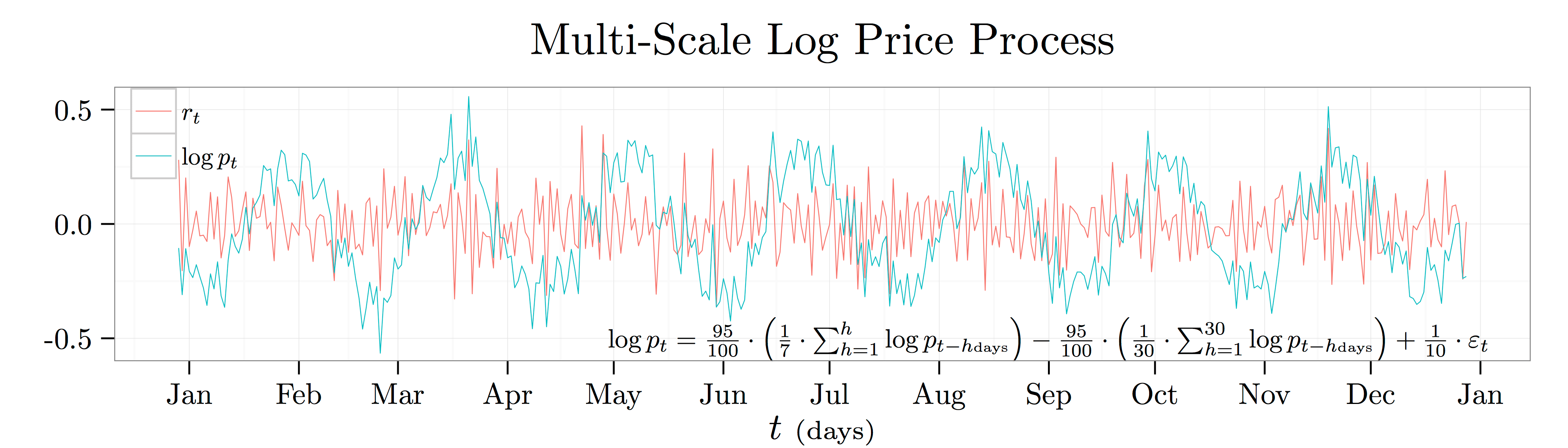
  in the time subscripts above because I want to emphasize the fact that the log price and return time series are scale dependent. In the analysis below, I’m going to think about running the analysis at the daily horizon so that
  .
.

 not
not  ) in the plot above. This process says that the log price today will go up by
  cents whenever the average log price over the last week was
![\begin{align*} \beta_h &= \frac{\mathrm{C}(h) \cdot \mathrm{StD}[\log p_t] \cdot \mathrm{StD}[\log p_{t-h}]}{\mathrm{Var}[\log p_{t-h}]} \quad \text{and} \quad \mathrm{StD}[\log p_t] = \mathrm{StD}[\log p_{t-h}] \end{align*}](https://alexchinco.com/wp-content/ql-cache/quicklatex.com-106e16135db2a7a4fdcdc8ab08aef998_l3.svg "Rendered by QuickLaTeX.com")
 can be written as the sum of
 is the completely deterministic time series and
  is the completely random white noise time series. The figure below shows the coefficient estimates,
  , from projecting the log price time series onto its past realizations for lags of anywhere from
  to
to  .
.

![\mathrm{T}_\theta[\cdot]](https://alexchinco.com/wp-content/ql-cache/quicklatex.com-71b99adc212b89da76131822264a0352_l3.svg "Rendered by QuickLaTeX.com") :
:![\begin{align*} \mathrm{T}_\theta[\mathrm{C}(h)] &= \mathrm{C}(h - \theta) \end{align*}](https://alexchinco.com/wp-content/ql-cache/quicklatex.com-81388b65dfdc423aeed598a2fc4233d1_l3.svg "Rendered by QuickLaTeX.com")
 time periods to the right. i.e., if
  gave you the autocorrelation between the log price at any two points in time that are
 ![\mathrm{T}_{1{\scriptscriptstyle \mathrm{day}}}[\mathrm{C}(4{\scriptstyle \mathrm{days}})]](https://alexchinco.com/wp-content/ql-cache/quicklatex.com-dd1d99221a5da52cfdcd9c5183467f19_l3.svg "Rendered by QuickLaTeX.com") would give you the autocorrelation between the log price at any two points in time that are
would give you the autocorrelation between the log price at any two points in time that are  :
:![\begin{align*} \mathrm{T}_\theta[\mathrm{C}_f(h)] &= \mathrm{C}_f(h - \theta) = \lambda_{f,\theta} \cdot \mathrm{C}_f(h) \end{align*}](https://alexchinco.com/wp-content/ql-cache/quicklatex.com-c49b84194f66b339d12de6cc71ae9967_l3.svg "Rendered by QuickLaTeX.com")
 and
and  .
.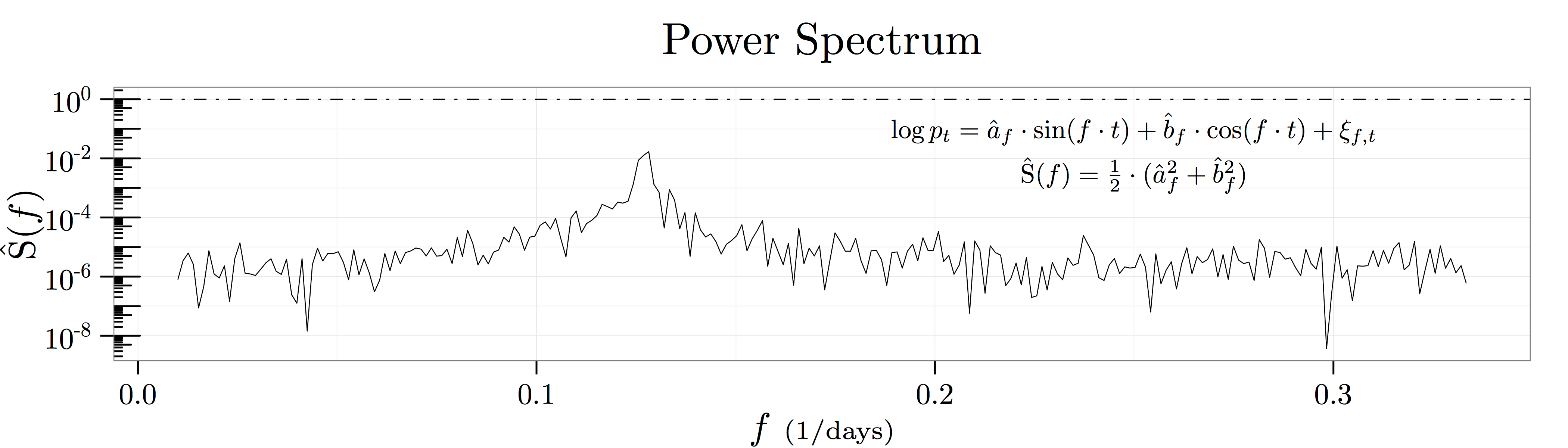
 as depicted in the figure above known as a spectral density plot. This figure shows the results of
 ![[1/100{\scriptstyle \mathrm{days}},1/3{\scriptstyle \mathrm{days}}]](https://alexchinco.com/wp-content/ql-cache/quicklatex.com-9c36912dbbc895ed4771ea183a1cf7db_l3.svg "Rendered by QuickLaTeX.com") :
:
 and
and  capture how predictive fluctuations at the frequency
  are of future log price movements. Thus, the summary statistic
  captures how much of the variation in log prices is explained by historical movements at the frequency
 and keeping only the real component yields the following mapping from frequency space to autocorrelation space:
![[0,F]](https://alexchinco.com/wp-content/ql-cache/quicklatex.com-e3f1473219fe5026f532e4a37a4e7bc4_l3.svg "Rendered by QuickLaTeX.com") covers a sufficient amount of the relevant frequency spectrum. The figure below verifies the mathematics by showing the close empirical fit between the two calculations.
covers a sufficient amount of the relevant frequency spectrum. The figure below verifies the mathematics by showing the close empirical fit between the two calculations.
 day moving average, there is no evidence of these
 . Likewise, the spectral density of the process shows a peak at somewhere between
  and
and  . Thus, the time scale we see in the raw data is an emergent feature of the interaction of both the weekly and monthly effects. Intuitively, it would be very hard to identify the economically relevant time scale from a stochastic process where interesting features emerge at all time scales.

 day, the equation above reads: “Daily changes in the log price are
  th of a percent, and these kicks have a half life of
  days.” Thus, it’s natural to think about this OU process as having a relevant time scale on the order of
  noise—i.e., noise which follows a power law decay pattern as shown in the figure below. Kicks which have a half life on the order of
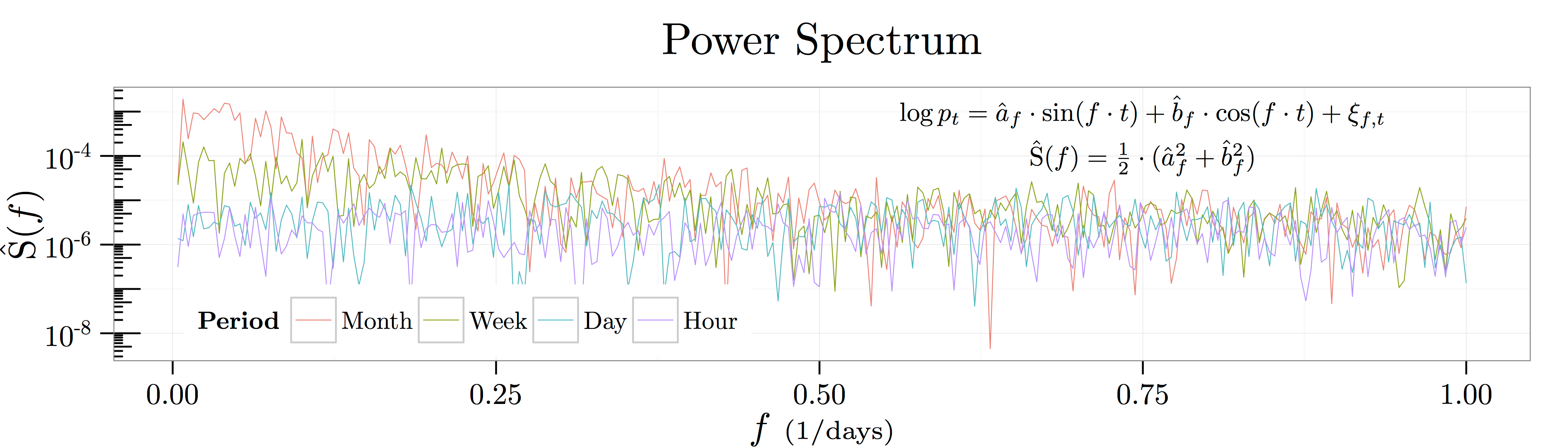

 as
as  if for each
  :
:
 , all of the coefficients
  are unique.

 and then empirically estimating
  . For each choice of approximations, I got a unique set of coefficients out. However, the counter example above in Section 5 shows that data generating functions with very different time scales can have very similar approximations. The analysis in this section shows that perhaps this result is not too surprising. A different way of putting this idea is that by choosing an approximation to data generating process,
  . If you are the social planner, you then try to maximize the benefits of having informative prices,
 ![\mathrm{Cov}[p,v]](https://alexchinco.com/wp-content/ql-cache/quicklatex.com-eea5550d0d75e112b760b018278b7cb4_l3.svg "Rendered by QuickLaTeX.com") , minus the costs of wasting lots of noise traders who could be doing other productive things,
, minus the costs of wasting lots of noise traders who could be doing other productive things,  , subject to the constraint that it has to be worth it for informed traders to enter into the market,
 ![\mathrm{E}[\text{informed trader profit}] \geq \bar{\pi}](https://alexchinco.com/wp-content/ql-cache/quicklatex.com-b4ac4f1b092c1bb35ccfea994f08980b_l3.svg "Rendered by QuickLaTeX.com") :
:![\begin{align*} \max_{\text{noise traders} \geq 0} \left\{ \mathrm{Cov}[p,v] - c(\text{noise traders}) \right\} \quad &\text{subject to} \quad \mathrm{E}[\text{informed trader profit}] \geq \bar{\pi} \end{align*}](https://alexchinco.com/wp-content/ql-cache/quicklatex.com-07f0a2c9a5e9b072d201ba6b7bba48bb_l3.svg "Rendered by QuickLaTeX.com")
![\begin{align*} \mathrm{Cov}[p,v] &= \text{constant} \times \sigma_v^2 \end{align*}](https://alexchinco.com/wp-content/ql-cache/quicklatex.com-3803994859ea15e9f1fdebd62fa5d682_l3.svg "Rendered by QuickLaTeX.com")
 , and will switch over to being butchers or bakers. However, pumping more and more noise traders into the market won’t make prices any more informative.
![\mathrm{Var}[v|s] = (1/\sigma_v^2 + 1/\sigma_\epsilon^2)^{-1}](https://alexchinco.com/wp-content/ql-cache/quicklatex.com-8282af7b3fe531628eca68ee914f05ab_l3.svg "Rendered by QuickLaTeX.com") and mean
and mean ![\mathrm{E}[v|s] = \mathrm{SNR} \cdot s](https://alexchinco.com/wp-content/ql-cache/quicklatex.com-7348a3664abdfcf84a86d3eba4fec598_l3.svg "Rendered by QuickLaTeX.com") where
where  denotes Alice’s signal to noise ratio:
 , directly then
  and here signal to noise ratio would be
  . Conversely, as
  her signal becomes meaningless and her signal to noise ratio tends to
  .
.![\begin{align*} y &= x + z \quad \text{where} \quad z \overset{\scriptscriptstyle \mathrm{iid}}{\sim} \mathrm{N}(0,\sigma_z^2) \\ p &= \mathrm{E}[v|y] \end{align*}](https://alexchinco.com/wp-content/ql-cache/quicklatex.com-47bc801618cd0fa1e4be8cb2e69624b0_l3.svg "Rendered by QuickLaTeX.com")
 denotes noise trader demand for Logs Inc stock. When I say that Bob only observes aggregate demand, I mean that if Bob sees a buy order of
  shares and the noise traders want to sell
 ![p = \mathrm{E}[v|y]](https://alexchinco.com/wp-content/ql-cache/quicklatex.com-49ec359e00b4b391d0822997f7018218_l3.svg "Rendered by QuickLaTeX.com") , someone else would step in and scoop his business.
, someone else would step in and scoop his business. :
:
 , and a pricing rule for Bob,
  , such that:
![\mathrm{E}[\pi_x|v]](https://alexchinco.com/wp-content/ql-cache/quicklatex.com-6a4417f24f1902198f4b5f7db9da221c_l3.svg "Rendered by QuickLaTeX.com") , yields an equation for her optimal demand given her realized signal,
, yields an equation for her optimal demand given her realized signal, 
 and
and  that govern Alice and Bob’s demand and pricing rules:
![\begin{align*} \lambda = \frac{\mathrm{Cov}[v,y]}{\mathrm{Var}[y]} &= \frac{\sqrt{\mathrm{SNR}}}{2} \cdot \frac{\sigma_v}{\sigma_z} \\ \beta = \frac{\mathrm{SNR}}{2 \cdot \lambda} &= \sqrt{\mathrm{SNR}} \cdot \frac{\sigma_z}{\sigma_v} \end{align*}](https://alexchinco.com/wp-content/ql-cache/quicklatex.com-fea5e9c2be9693136b07048424725a38_l3.svg "Rendered by QuickLaTeX.com")
 means that the price of Logs Inc stock will be more responsive to aggregate demand shocks when there is more information to be revealed or when there are few noise traders to mask the information. Conversely, Alice’s demand will be more responsive to a strong private signal when there is more noise trading for her to hid behind or when she wasn’t expecting to discover much in the first place.
 , doesn’t have any dependence on the number of noise traders in the market. i.e., if the fundamental value of Logs Inc goes up by
  , then the price of Logs Inc will go up by
  on average, and this relationship will be true whether the volatility of noise trader demand is
 ![\begin{align*} \mathrm{Cov}[p,v] &= \frac{\mathrm{SNR}}{2} \cdot \sigma_v^2 \end{align*}](https://alexchinco.com/wp-content/ql-cache/quicklatex.com-73b0b9d55d662bb9fb3ffe6ed330fdf9_l3.svg "Rendered by QuickLaTeX.com")
![\begin{align*} \mathrm{E}[\pi_x] &= - \mathrm{E}[\pi_z] = \frac{\sqrt{\mathrm{SNR}}}{2} \cdot \sigma_z \cdot \sigma_v \end{align*}](https://alexchinco.com/wp-content/ql-cache/quicklatex.com-c0bea7042127f7b6b083258abe39a2a0_l3.svg "Rendered by QuickLaTeX.com")
 . It might be worth it if it’s really helpful for everyone in the economy to see an accurate valuation of Logs Inc. There are lots of transfer payments which people are happy to make (e.g., welfare, social security, etc…), but the key observation is that it’s a transfer payment. What’s more, since adding more noise traders doesn’t affect price informativeness, you are going to want to sacrifice the the minimum number of noise trader required to make sure that Alice is a trader and not a butcher:
 , so that total noise trader demand variance is given by
  .
.

 . e.g., if
  then he would believe that fundamental volatility was
  when it was in fact
  . When Alice gets a really strong signal abou the fundamental value,
 ![\begin{align*} \mathrm{Cov}[p,v] &= \frac{1}{2} \cdot \sigma_v^2 \cdot \left\{ 1 + \eta + \eta^2 + \cdots \right\} \end{align*}](https://alexchinco.com/wp-content/ql-cache/quicklatex.com-62df12d59bcb04e6b18c4eeca2953cc3_l3.svg "Rendered by QuickLaTeX.com")
 , problems can occur and the delicate balance between
 ![\begin{align*} \mathrm{Cov}[p,v] &= \frac{\mathrm{SNR}}{2} \cdot \sigma_v^2 \cdot \left\{ 1 + \eta \cdot (2 - \mathrm{SNR}) + \cdots \right\} \end{align*}](https://alexchinco.com/wp-content/ql-cache/quicklatex.com-0a036c3a29e80e8540eb50c10d22115e_l3.svg "Rendered by QuickLaTeX.com")
 , the factor multiplying
  is greater than unity. Thus, when Alice gets really weak signals about the fundamental value of Logs Inc, minor errors in Bob’s understanding of the market can lead to wildly incorrect pricing.
You must be logged in to post a comment.