1. Introduction
Imagine you are an algorithmic trader, and you have to set up a trading platform. How many signals should you try to process? How many assets should you trade? If you are like most people, your answer will be something like: “As many as I possibly can given my technological constraints.” Most people have the intuition that the only thing holding back algorithmic trading is computational speed. They think that left unchecked, computers will eventually uncover every trading opportunity no matter how small or obscure. e.g., as Scott Patterson writes in Dark Pools, these computerized trading platforms are just “tricked-out artificial intelligence systems designed to scope out hidden pockets in the market where they can ply their trades.”
This post highlights another concern. As you use computers to discover more and more “hidden pockets in the market”, the scale of these trades might grow faster than the usefulness of your information. Weak and diffuse signals might turn out to be really risky to trade on. How might this work? e.g., suppose that in order for your computers to recognize the impact of China’s GDP on US stock returns you need to feed them data for  assets; however, in order for your computers to recognize the impact of recent copper discoveries in Guatemala on electronics manufacturing company returns, you need to feed your machines data on
  assets. Even if the precision of the signal that your computers spit out is the same, its magnitude will be smaller. Copper discoveries in Guatemala just don’t matter as much. Thus, you would take on more risk by aggressively trading the second signal because it’s weaker and you would have to take on a position in
  times as many assets! Thus, this post suggests that even if you might want to maximize the number of inputs your machines get, you might want to limit how broadly you apply them.
First, in Section 2 I illustrate how the scale of a trading opportunity might increase faster than the precision on your signal via an an example based on the well known Hodges’ Estimator. You should definitely check out Larry Wasserman‘s excellent post on the this topic for an introduction to the ideas. In Section 3 I then outline the basic decision problem I have in mind. In Section 4 I show how the risk associated with trading weak signals might explode as described above. Finally, in Section 4 I conclude by suggesting an empirical application of these ideas.
2. Hodges’ Estimator
Think about the following problem. Suppose that  are random variables denoting (say) innovations in the quarterly dividends of a group of
  stocks:
(1) ![\begin{align*} m_q &= d_{q,t+1} - \mathrm{E}_t[d_{q,t+1}] \end{align*}](https://alexchinco.com/wp-content/ql-cache/quicklatex.com-21af1155fde5369169b652a47faeb340_l3.svg "Rendered by QuickLaTeX.com")
You want to know if the mean of the dividend changes is non-zero. i.e., has this group of stocks realized a shock? Define the estimator ![\mathrm{Hdg}[Q]](https://alexchinco.com/wp-content/ql-cache/quicklatex.com-8ed4fbe1cfbe188f08b690e7164d5ae1_l3.svg "Rendered by QuickLaTeX.com") as follows:
as follows:
(2) ![\begin{align*} \mathrm{Hdg}[Q] &= \begin{cases} \mathrm{Avg}[Q] &\text{if } \mathrm{Avg}[Q] \geq Q^{-1/4} \\ 0 &\text{else } \end{cases} \end{align*}](https://alexchinco.com/wp-content/ql-cache/quicklatex.com-a9f917f42b8a294d98fa9f5aab0187d1_l3.svg "Rendered by QuickLaTeX.com")
where ![\mathrm{Avg}[Q] = \frac{1}{Q} \cdot \sum_{q=1}^Q m_q](https://alexchinco.com/wp-content/ql-cache/quicklatex.com-8c1429353451423eeadae3e7e0f1ff46_l3.svg "Rendered by QuickLaTeX.com") . This estimator says: “If the average of the dividend changes is sufficiently big, I’m going to assume there has been a shock of size
. This estimator says: “If the average of the dividend changes is sufficiently big, I’m going to assume there has been a shock of size ![\mathrm{Avg}[Q]](https://alexchinco.com/wp-content/ql-cache/quicklatex.com-5e63a24032eab3839810285abade57a4_l3.svg "Rendered by QuickLaTeX.com") ; otherwise, I’ll assume that there’s been no shock.” This is an example of a Hodges-type estimator. is a consistent estimator of
; otherwise, I’ll assume that there’s been no shock.” This is an example of a Hodges-type estimator. is a consistent estimator of  in the sense that:
(3) ![\begin{align*} \sqrt{Q} \cdot (\mathrm{Hdg}[Q] - \mu) &\overset{\scriptscriptstyle \mathrm{Dist}}{\to} \begin{cases} N(0,1) &\text{if } \mu \neq 0 \\ 0 &\text{if } \mu = 0 \end{cases} \end{align*}](https://alexchinco.com/wp-content/ql-cache/quicklatex.com-eb0e1c8ebb81cfde73fa88a730bb8280_l3.svg "Rendered by QuickLaTeX.com")
Thus, as you examine more and more stocks from this group, you are guaranteed to discover the true mean. However, the worst case expected loss of the estimator, , is infinite!
(4) ![\begin{align*} \sup_\mu \mathrm{E}\left[ Q \cdot (\mathrm{Hdg}[Q] - \mu)^2 \right] &\to \infty \end{align*}](https://alexchinco.com/wp-content/ql-cache/quicklatex.com-d379a6f2fa329ad600c19b82c37e1645_l3.svg "Rendered by QuickLaTeX.com")
This is true even though the worst case loss for the sample mean, , is flat:
(5) ![\begin{align*} \sup_\mu \mathrm{E}\left[ Q \cdot (\mathrm{Avg}[Q] - \mu)^2 \right] &\to 1 \end{align*}](https://alexchinco.com/wp-content/ql-cache/quicklatex.com-01adaff2f0fd5dbf3920a3fcd8c87367_l3.svg "Rendered by QuickLaTeX.com")
I plot the risk associated with Hodges’ estimator in the figure below. What’s going on here? Well, as gets bigger and bigger, there remains a region around  where you are quite certain that the mean is
  . However, at the edge of this region, there is a band of values of where if you are wrong and
  , then your prediction error summed across every one of the stocks you examined turns out to be quite big.

3. Decision Problem
Now, think about a decision problem that generates a really similar decision rule—namely, try to figure out how many shares,  , to purchase where the stock’s payout is determined by
  different attributes via the coefficients
  :
:
(6) 
Here, you are trying to maximize your value,  , by choosing the right number of shares to hold—i.e., the risk action. Ideally you would take the action which is exactly equal to the ideal action
  ; however, it’s hard to figure out the exact loadings, , for every single one of the relevant dimensions. As a result, you take an action which isn’t exactly perfect:
(7) 
I use the function  to denote the loss in value you suffer by choosing a suboptimal asset holding:
(8) ![\begin{align*} L(\mathbf{m};{\boldsymbol \mu}) = L(\mathbf{m}) &= \mathrm{E}\left[ \ V(A({\boldsymbol \mu}); {\boldsymbol \mu}, \mathbf{x}) - V(A(\mathbf{m}); {\boldsymbol \mu}, \mathbf{x}) \ \right] \\ &= - \frac{\gamma}{2} \cdot \mathrm{E}\left[ \left( \sum_{n=1}^N (m_n - \mu_n) \cdot x_n \right)^2 \right] \\ &= \frac{\gamma}{2} \cdot \mathrm{E}\left[ \sum_{n=1}^N (m_n - \mu_n)^2 \right] \end{align*}](https://alexchinco.com/wp-content/ql-cache/quicklatex.com-52108ba53b21d3e6ba0798bb5980f8cf_l3.svg "Rendered by QuickLaTeX.com")
where the  rd line follows from assuming that
  .
.
So which of the different details should you pay attention to? Which of them should you ignore? One way to frame this problem would be to look for a sparse solution and only ask your computers to trade on the signals that are sufficiently important. Gabaix (2012) shows how to do this using an  -program, I outline the main ideas in an earlier post. Basically, you would try to minimize your loss from taking a suboptimal action subject to an -penalty:
(9) 
so that your optimal choice of actions is given by:
(10) 
That’s the decision problem. So far everything is old hat.
4. Maximum Risk
The key insight in this post is that these  terms don’t come down from on high. As a trader, you don’t just know what these terms are from the outset. They weren’t stitched onto the forehead of your favorite teddy bear. Instead, you have to use data on lots of stocks to estimate them as you go. In this section, I think about a world where you feed data on different stocks to your machines, and each of these assets has the appropriate action
  . I then investigate what happens when you use the estimator:
(11) ![\begin{align*} \widetilde{m}_n &= \begin{cases} \mathrm{Avg}_n[Q] &\text{if } |\mathrm{Avg}_n[Q]| \geq \kappa \\ 0 &\text{if } |\mathrm{Avg}_n[Q]| < \kappa \end{cases} \end{align*}](https://alexchinco.com/wp-content/ql-cache/quicklatex.com-098f34f9475cfc607ed8ec034305cec9_l3.svg "Rendered by QuickLaTeX.com")
instead of the estimator in Equation (10) where ![\mathrm{Avg}_n[Q] = \frac{1}{Q} \cdot \sum_{q=1}^Q \mu_{n,q}](https://alexchinco.com/wp-content/ql-cache/quicklatex.com-1561027d49ea48756f3e35a4d5ffc346_l3.svg "Rendered by QuickLaTeX.com") and
and  isn’t growing that fast as gets larger and larger. i.e., we have that:
(12) ![\begin{align*} \widetilde{m}_n &= \mathrm{Avg}_n[Q] \cdot 1_{\{ |\mathrm{Avg}_n[Q]| \geq \kappa \}} \quad \text{with} \quad \kappa = \mathrm{O}(\sqrt{2 \log Q}) \end{align*}](https://alexchinco.com/wp-content/ql-cache/quicklatex.com-53f7931263f20a0006456f7fad0a017f_l3.svg "Rendered by QuickLaTeX.com")
In some senses,  is still a really good estimator of . To see this, let denote the true effect for a particular attribute. Then, clearly for
  , we have that:
(13) 
Similarly, for  , we have that:
(14) 
Thus, the estimate  is a strictly better estimator of than the sample average. Pretty cool.
However, in another sense, it’s a terrible estimator since the maximum risk associated with trading on is unbounded:
(15) ![\begin{align*} \sup_{\mu_n} R_n(\widetilde{\mathbf{m}}) &\to \infty \quad \text{where} \quad R_n(\widetilde{\mathbf{m}}) = \mathrm{E}\left[ Q \cdot (\widetilde{m}_n - \mu_n)^2 \right] \end{align*}](https://alexchinco.com/wp-content/ql-cache/quicklatex.com-9123948c0686bb8e5fb321fc160056fc_l3.svg "Rendered by QuickLaTeX.com")
This result means that if you use this estimator to trade on, there are parameter values for which lead your computer to take on positions that are infinitely risky and make you really unhappy! How is this possible? Well, take a look at the following decomposition of the risk associated with the estimator :
(16) ![\begin{align*} R_n(\widetilde{\mathbf{m}}) &= \mathrm{E}\left[ Q \cdot (\widetilde{m}_n - \mu_n)^2 \right] \\ &= \mathrm{E}\left[ Q \cdot (\mathrm{Avg}_n[Q] \cdot 1_{\{ |\mathrm{Avg}_n[Q]| \geq \kappa \}} - \mu_n)^2 \right] \\ &= \mathrm{Pr}\left[ |\mathrm{Avg}_n[Q]| \geq \kappa \right] \cdot \mathrm{E}\left[ Q \cdot (\mathrm{Avg}_n[Q] - \mu_n)^2 \right] + \mathrm{Pr}\left[ |\mathrm{Avg}_n[Q]| < \kappa \right] \cdot \mathrm{E}\left[ Q \cdot \mu_n^2 \right] \end{align*}](https://alexchinco.com/wp-content/ql-cache/quicklatex.com-cf7fd7fba9f52154e16b4175419d7703_l3.svg "Rendered by QuickLaTeX.com")
It turns out that there are choices of for which ![\mathrm{Pr}\left[ |\mathrm{Avg}_n[Q]| < \kappa \right] \to 1](https://alexchinco.com/wp-content/ql-cache/quicklatex.com-409849c197f7bd39bde826bddfa5664c_l3.svg "Rendered by QuickLaTeX.com") as
as  , but at the same time
 ![\mathrm{E}\left[ Q \cdot \mu_n^2 \right] \to \infty](https://alexchinco.com/wp-content/ql-cache/quicklatex.com-b360b7333eddfaca05ab089e100fcc4f_l3.svg "Rendered by QuickLaTeX.com") for the same process. In words, this means that there are choices of which make dimension
for the same process. In words, this means that there are choices of which make dimension  always appear to your machines as an unimportant detail no matter how many stocks you look at, but this conclusion is still risky enough that if you applied to every one of these stocks you’d get an infinitely risky portfolio.
e.g., consider the case where:
(17) 
Then, it’s easy to see that:
(18) ![\begin{align*} \mathrm{Pr}_{\mu_n} \left[ \ |\mathrm{Avg}_n[Q]| < Q^{-1/4} \ \right] &= \mathrm{Pr}_{\mu_n} \left[ \ Q^{-1/4} < \mathrm{Avg}_n[Q] < Q^{-1/4} \ \right] \\ &= \mathrm{Pr}_{\mu_n} \left[ \ \sqrt{Q} \cdot \left(- Q^{-1/4} - \mu_n \right) < z < \sqrt{Q} \cdot \left(- Q^{-1/4} - \mu_n \right) \ \right] \\ &= \mathrm{Pr}_{\mu_n} \left[ \ - Q^{1/4} \cdot ( 1 + \hbar ) < z < Q^{1/4} \cdot ( 1 - \hbar ) \ \right] \end{align*}](https://alexchinco.com/wp-content/ql-cache/quicklatex.com-d131f80b030d3f0933d925b8b522987a_l3.svg "Rendered by QuickLaTeX.com")
where  . But, this means that as , we have that:
(19) ![\begin{align*} \mathrm{Pr}_{\mu_n} \left[ \mathrm{Avg}_n[Q] < \kappa \right] &\to 1 \quad \text{while} \quad \mathrm{E}\left[ Q \cdot \mu_n^2 \right] \to \infty \end{align*}](https://alexchinco.com/wp-content/ql-cache/quicklatex.com-ddc54b5aa8cc71a5bb60e6e848ff3f04_l3.svg "Rendered by QuickLaTeX.com")
Thus, we have a proof by explicit construction. The punchline is that unleashing your machines on the market might lead them into situations where the scale of the position grows faster than the precision of the signal.
5. Empirical Prediction
What does this result mean in the real world? Well, the argument in the section above relied on the fact that when you used different assets to derive a signal, you also then traded on all assets. i.e., this is why the risk function has a factor of in it. Thus, one way to get around this problem would be to commit to trading a smaller number of asset  where:
(20) 
even though you had to use assets to recover the signal. i.e., even if you have to grab signals from the  corners of the market to create your trading strategy, you might nevertheless specialize in trading only a few assets so that in contrast to Equation (19) you would always have:
(21) ![\begin{align*} \mathrm{Pr}_{\mu_n} \left[ \mathrm{Avg}_n[Q] < \kappa \right] &\to 1 \quad \text{while} \quad \mathrm{E}\left[ Q' \cdot \mu_n^2 \right] \to \mathrm{const} < \infty \end{align*}](https://alexchinco.com/wp-content/ql-cache/quicklatex.com-abcaf1f97810ee9545d6d87aa9059b7b_l3.svg "Rendered by QuickLaTeX.com")
If traders are actually using signals from lots of assets, but only trading a few of them to avoid the infinite risk problem, then this theory would give a new motivation for excess comovement. i.e., you and I might feed the same data into our machines, get the same output, and choose to trade on entirely different subsets of stocks.
 to
to  . What’s more, the red vertical lines in the top figure show the intraday range for the traded price, and these bands stretch
  per share in some cases. People are trading this ETF at all sorts of different investment horizons. Any model fit to daily data will ignore really interesting economics operating at these shorter investment horizons. Vice versa, any model fit to higher frequency minute-by-minute data will miss out on some longer buy-and-hold decisions.
 sections discuss different ways of recovering the relevant time scales from a financial data series. In particular, I am interested in the time series of log prices as I don’t want to have to worry about the series going negative. I define returns,
  , as:
, as:
![\begin{align*} \mathrm{E}[x_t] &= 0 \quad \text{and} \quad \mathrm{E}[x_t \cdot x_{t - h \cdot \Delta t}] = \mathrm{C}(h) \cdot \sigma^2 \end{align*}](https://alexchinco.com/wp-content/ql-cache/quicklatex.com-189e908a8df39756af726aa96820a7cb_l3.svg "Rendered by QuickLaTeX.com")
 where
where  denotes the
  -period ahead autocorrelation function. I use
  instead of the usual
  in the time subscripts above because I want to emphasize the fact that the log price and return time series are scale dependent. In the analysis below, I’m going to think about running the analysis at the daily horizon so that
  .
.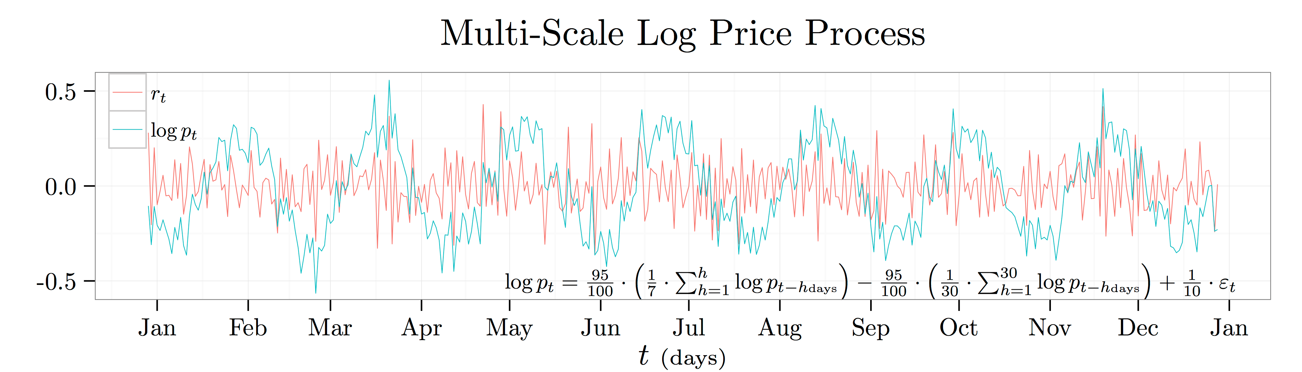

 not
not  ) in the plot above. This process says that the log price today will go up by
  cents whenever the average log price over the last week was
  unit higher, but it will go down by
![\begin{align*} \beta_h &= \frac{\mathrm{C}(h) \cdot \mathrm{StD}[\log p_t] \cdot \mathrm{StD}[\log p_{t-h}]}{\mathrm{Var}[\log p_{t-h}]} \quad \text{and} \quad \mathrm{StD}[\log p_t] = \mathrm{StD}[\log p_{t-h}] \end{align*}](https://alexchinco.com/wp-content/ql-cache/quicklatex.com-106e16135db2a7a4fdcdc8ab08aef998_l3.svg "Rendered by QuickLaTeX.com")
 can be written as the sum of
 is the completely deterministic time series and
  is the completely random white noise time series. The figure below shows the coefficient estimates,
  , from projecting the log price time series onto its past realizations for lags of anywhere from
  to
to  .
.

![\mathrm{T}_\theta[\cdot]](https://alexchinco.com/wp-content/ql-cache/quicklatex.com-71b99adc212b89da76131822264a0352_l3.svg "Rendered by QuickLaTeX.com") :
:![\begin{align*} \mathrm{T}_\theta[\mathrm{C}(h)] &= \mathrm{C}(h - \theta) \end{align*}](https://alexchinco.com/wp-content/ql-cache/quicklatex.com-81388b65dfdc423aeed598a2fc4233d1_l3.svg "Rendered by QuickLaTeX.com")
 time periods to the right. i.e., if
  gave you the autocorrelation between the log price at any two points in time that are
 ![\mathrm{T}_{1{\scriptscriptstyle \mathrm{day}}}[\mathrm{C}(4{\scriptstyle \mathrm{days}})]](https://alexchinco.com/wp-content/ql-cache/quicklatex.com-dd1d99221a5da52cfdcd9c5183467f19_l3.svg "Rendered by QuickLaTeX.com") would give you the autocorrelation between the log price at any two points in time that are
would give you the autocorrelation between the log price at any two points in time that are  :
:![\begin{align*} \mathrm{T}_\theta[\mathrm{C}_f(h)] &= \mathrm{C}_f(h - \theta) = \lambda_{f,\theta} \cdot \mathrm{C}_f(h) \end{align*}](https://alexchinco.com/wp-content/ql-cache/quicklatex.com-c49b84194f66b339d12de6cc71ae9967_l3.svg "Rendered by QuickLaTeX.com")
 and
and  .
.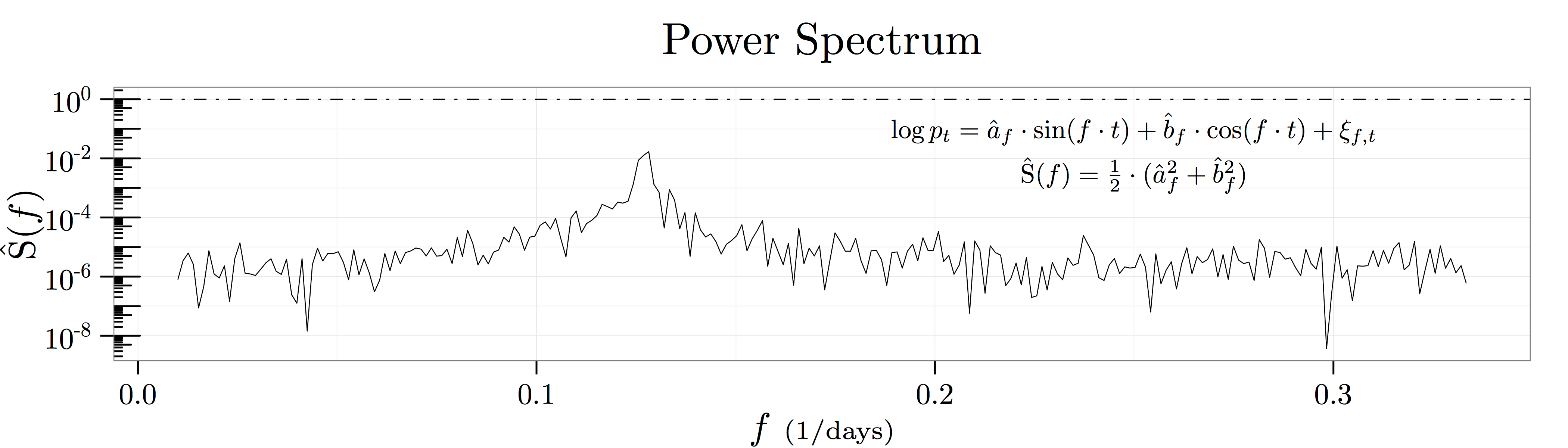
 as depicted in the figure above known as a spectral density plot. This figure shows the results of
  regressions at frequencies in the range
 ![[1/100{\scriptstyle \mathrm{days}},1/3{\scriptstyle \mathrm{days}}]](https://alexchinco.com/wp-content/ql-cache/quicklatex.com-9c36912dbbc895ed4771ea183a1cf7db_l3.svg "Rendered by QuickLaTeX.com") :
:
 and
and  capture how predictive fluctuations at the frequency
  in units of
  are of future log price movements. Thus, the summary statistic
  captures how much of the variation in log prices is explained by historical movements at the frequency
 and keeping only the real component yields the following mapping from frequency space to autocorrelation space:
![[0,F]](https://alexchinco.com/wp-content/ql-cache/quicklatex.com-e3f1473219fe5026f532e4a37a4e7bc4_l3.svg "Rendered by QuickLaTeX.com") covers a sufficient amount of the relevant frequency spectrum. The figure below verifies the mathematics by showing the close empirical fit between the two calculations.
covers a sufficient amount of the relevant frequency spectrum. The figure below verifies the mathematics by showing the close empirical fit between the two calculations.
 day moving average and a
  day moving average, there is no evidence of these
 . Likewise, the spectral density of the process shows a peak at somewhere between
  and
and  . Thus, the time scale we see in the raw data is an emergent feature of the interaction of both the weekly and monthly effects. Intuitively, it would be very hard to identify the economically relevant time scale from a stochastic process where interesting features emerge at all time scales.

 day, the equation above reads: “Daily changes in the log price are
  th of a percent, and these kicks have a half life of
  days.” Thus, it’s natural to think about this OU process as having a relevant time scale on the order of
  noise—i.e., noise which follows a power law decay pattern as shown in the figure below. Kicks which have a half life on the order of
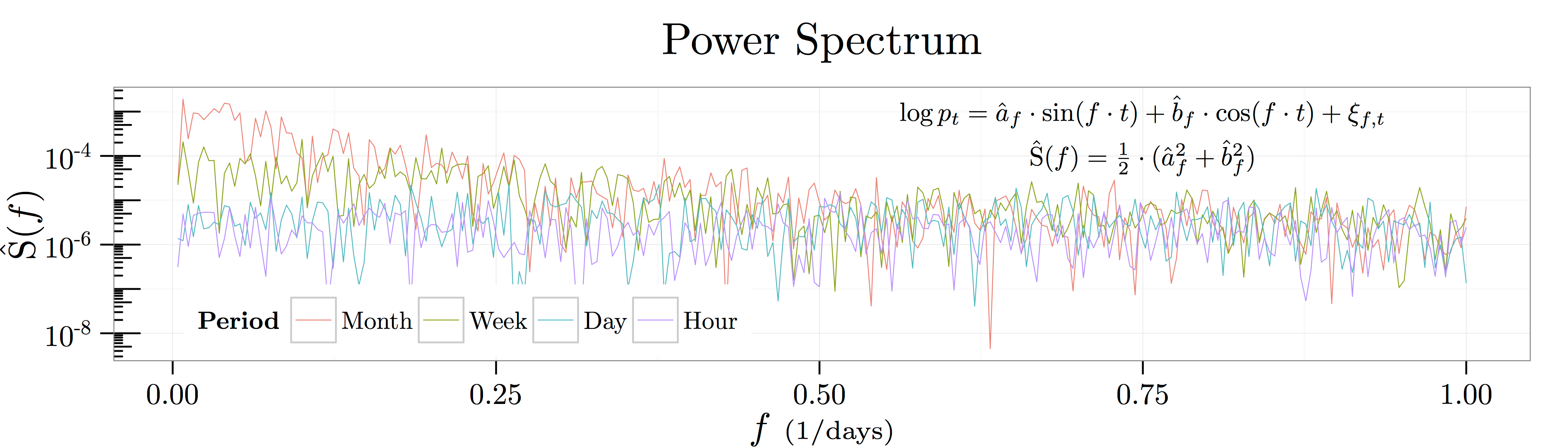

 as
as  if for each
  :
:
 , all of the coefficients
  are unique.

 and then empirically estimating
  . For each choice of approximations, I got a unique set of coefficients out. However, the counter example above in Section 5 shows that data generating functions with very different time scales can have very similar approximations. The analysis in this section shows that perhaps this result is not too surprising. A different way of putting this idea is that by choosing an approximation to data generating process,
  and has price
  . If you are the social planner, you then try to maximize the benefits of having informative prices,
 ![\mathrm{Cov}[p,v]](https://alexchinco.com/wp-content/ql-cache/quicklatex.com-eea5550d0d75e112b760b018278b7cb4_l3.svg "Rendered by QuickLaTeX.com") , minus the costs of wasting lots of noise traders who could be doing other productive things,
, minus the costs of wasting lots of noise traders who could be doing other productive things,  , subject to the constraint that it has to be worth it for informed traders to enter into the market,
 ![\mathrm{E}[\text{informed trader profit}] \geq \bar{\pi}](https://alexchinco.com/wp-content/ql-cache/quicklatex.com-b4ac4f1b092c1bb35ccfea994f08980b_l3.svg "Rendered by QuickLaTeX.com") :
:![\begin{align*} \max_{\text{noise traders} \geq 0} \left\{ \mathrm{Cov}[p,v] - c(\text{noise traders}) \right\} \quad &\text{subject to} \quad \mathrm{E}[\text{informed trader profit}] \geq \bar{\pi} \end{align*}](https://alexchinco.com/wp-content/ql-cache/quicklatex.com-07f0a2c9a5e9b072d201ba6b7bba48bb_l3.svg "Rendered by QuickLaTeX.com")
![\begin{align*} \mathrm{Cov}[p,v] &= \text{constant} \times \sigma_v^2 \end{align*}](https://alexchinco.com/wp-content/ql-cache/quicklatex.com-3803994859ea15e9f1fdebd62fa5d682_l3.svg "Rendered by QuickLaTeX.com")
 , and will switch over to being butchers or bakers. However, pumping more and more noise traders into the market won’t make prices any more informative.
 , about the fundamental value of a lumber company, Logs Inc:
![\mathrm{Var}[v|s] = (1/\sigma_v^2 + 1/\sigma_\epsilon^2)^{-1}](https://alexchinco.com/wp-content/ql-cache/quicklatex.com-8282af7b3fe531628eca68ee914f05ab_l3.svg "Rendered by QuickLaTeX.com") and mean
and mean ![\mathrm{E}[v|s] = \mathrm{SNR} \cdot s](https://alexchinco.com/wp-content/ql-cache/quicklatex.com-7348a3664abdfcf84a86d3eba4fec598_l3.svg "Rendered by QuickLaTeX.com") where
where  denotes Alice’s signal to noise ratio:
 , directly then
  and here signal to noise ratio would be
  . Conversely, as
  her signal becomes meaningless and her signal to noise ratio tends to
  .
. , and sets the price equal to his conditional expectation of its fundamental value:
![\begin{align*} y &= x + z \quad \text{where} \quad z \overset{\scriptscriptstyle \mathrm{iid}}{\sim} \mathrm{N}(0,\sigma_z^2) \\ p &= \mathrm{E}[v|y] \end{align*}](https://alexchinco.com/wp-content/ql-cache/quicklatex.com-47bc801618cd0fa1e4be8cb2e69624b0_l3.svg "Rendered by QuickLaTeX.com")
 denotes Alice’s informed demand for Logs Inc stock in units of shares and
  denotes noise trader demand for Logs Inc stock. When I say that Bob only observes aggregate demand, I mean that if Bob sees a buy order of
  shares and the noise traders want to sell
 ![p = \mathrm{E}[v|y]](https://alexchinco.com/wp-content/ql-cache/quicklatex.com-49ec359e00b4b391d0822997f7018218_l3.svg "Rendered by QuickLaTeX.com") , someone else would step in and scoop his business.
, someone else would step in and scoop his business. :
:
 , and a pricing rule for Bob,
  , such that:
![\mathrm{E}[\pi_x|v]](https://alexchinco.com/wp-content/ql-cache/quicklatex.com-6a4417f24f1902198f4b5f7db9da221c_l3.svg "Rendered by QuickLaTeX.com") , yields an equation for her optimal demand given her realized signal,
, yields an equation for her optimal demand given her realized signal, 
 and
and  that govern Alice and Bob’s demand and pricing rules:
![\begin{align*} \lambda = \frac{\mathrm{Cov}[v,y]}{\mathrm{Var}[y]} &= \frac{\sqrt{\mathrm{SNR}}}{2} \cdot \frac{\sigma_v}{\sigma_z} \\ \beta = \frac{\mathrm{SNR}}{2 \cdot \lambda} &= \sqrt{\mathrm{SNR}} \cdot \frac{\sigma_z}{\sigma_v} \end{align*}](https://alexchinco.com/wp-content/ql-cache/quicklatex.com-fea5e9c2be9693136b07048424725a38_l3.svg "Rendered by QuickLaTeX.com")
 means that the price of Logs Inc stock will be more responsive to aggregate demand shocks when there is more information to be revealed or when there are few noise traders to mask the information. Conversely, Alice’s demand will be more responsive to a strong private signal when there is more noise trading for her to hid behind or when she wasn’t expecting to discover much in the first place.
 , doesn’t have any dependence on the number of noise traders in the market. i.e., if the fundamental value of Logs Inc goes up by
  , then the price of Logs Inc will go up by
  on average, and this relationship will be true whether the volatility of noise trader demand is
  shares per period or
 ![\begin{align*} \mathrm{Cov}[p,v] &= \frac{\mathrm{SNR}}{2} \cdot \sigma_v^2 \end{align*}](https://alexchinco.com/wp-content/ql-cache/quicklatex.com-73b0b9d55d662bb9fb3ffe6ed330fdf9_l3.svg "Rendered by QuickLaTeX.com")
![\begin{align*} \mathrm{E}[\pi_x] &= - \mathrm{E}[\pi_z] = \frac{\sqrt{\mathrm{SNR}}}{2} \cdot \sigma_z \cdot \sigma_v \end{align*}](https://alexchinco.com/wp-content/ql-cache/quicklatex.com-c0bea7042127f7b6b083258abe39a2a0_l3.svg "Rendered by QuickLaTeX.com")
 . It might be worth it if it’s really helpful for everyone in the economy to see an accurate valuation of Logs Inc. There are lots of transfer payments which people are happy to make (e.g., welfare, social security, etc…), but the key observation is that it’s a transfer payment. What’s more, since adding more noise traders doesn’t affect price informativeness, you are going to want to sacrifice the the minimum number of noise trader required to make sure that Alice is a trader and not a butcher:
 , so that total noise trader demand variance is given by
  .
.

 . e.g., if
  then he would believe that fundamental volatility was
  when it was in fact
  . When Alice gets a really strong signal abou the fundamental value,
 ![\begin{align*} \mathrm{Cov}[p,v] &= \frac{1}{2} \cdot \sigma_v^2 \cdot \left\{ 1 + \eta + \eta^2 + \cdots \right\} \end{align*}](https://alexchinco.com/wp-content/ql-cache/quicklatex.com-62df12d59bcb04e6b18c4eeca2953cc3_l3.svg "Rendered by QuickLaTeX.com")
 , problems can occur and the delicate balance between
 ![\begin{align*} \mathrm{Cov}[p,v] &= \frac{\mathrm{SNR}}{2} \cdot \sigma_v^2 \cdot \left\{ 1 + \eta \cdot (2 - \mathrm{SNR}) + \cdots \right\} \end{align*}](https://alexchinco.com/wp-content/ql-cache/quicklatex.com-0a036c3a29e80e8540eb50c10d22115e_l3.svg "Rendered by QuickLaTeX.com")
 , the factor multiplying
  is greater than unity. Thus, when Alice gets really weak signals about the fundamental value of Logs Inc, minor errors in Bob’s understanding of the market can lead to wildly incorrect pricing.
 to exploit the momentum anomaly at the monthly horizon. This position has a price of
  dollars, and costs Mr. Market
  dollars to put together. You and Mr. Market split the gains to trade with you getting a fraction,
  , and Mr. Market getting a fraction,
  , so that:
 , your boiler-plate portfolio position
  dollars where
  . In this situation, you actually need to put together the position
  to exploit momentum while staying market neutral. Portfolio
  dollars. For example, during the Quant Crisis of August 2007 the market suddenly and unexpectedly went sideways for quantitative traders in long-short equity positions. According to
  to
to  ” of assets under management.
 denotes the probability that you discover the correct portfolio position
 -dimensional vector,
 ![\begin{align*} \widetilde{\mathrm{E}}[\mathbf{x}^{\top} \mathbf{a}] &= p \end{align*}](https://alexchinco.com/wp-content/ql-cache/quicklatex.com-3b85b82e638c1aa9f1a61f4ef3f556f4_l3.svg "Rendered by QuickLaTeX.com")
 denotes the
  th of your portfolio holdings each month at a total price of
  months.
 your initial ideas about how the market will play out turn out to be wrong, and the portfolio position
 . For example, if you are the only trader in the market trying to sell the stocks required by portfolio
  . Here,
  of the time, then
  and you would be
  dollars in cognitive costs to maintain this level of informativeness. I assume both that:


 , times the probability that you didn’t discover this fact during your search,
  . The denominator is the probability that you didn’t find an alternative portfolio,
  . If
. If 
 dollars is the surplus available to be split after realizing ex post that
  denote your equilibrium level of search. The ex ante price
  for portfolio

 . If you conceal
  where the middle term comes from the fact that you know you will have to rebalance your portfolio and the price is given by Equation (
 . The important thing about Equation (
 :
:
 , any investment in cognition is purely rent-seeking!
![\begin{align*} U_{\mathrm{Trader}} &= \max_{\pi \in [0,1]} \Big\{ \rho \cdot \pi \cdot \theta_{\mathrm{Trader}} \cdot (v - c_{\mathrm{Transact}}) \\ &\qquad \qquad \qquad + \ \rho \cdot (1 - \pi) \cdot \left\{ v - (c_{\mathrm{Rebal}} + h) - p(\pi^*)\right\} \\ &\qquad \qquad \qquad \qquad + \ (1 - \rho) \cdot \left\{ v - p(\pi^*) \right\} \\ &\qquad \qquad \qquad \qquad \qquad - \ \mathrm{Eff}(\pi) \Big\} \end{align*}](https://alexchinco.com/wp-content/ql-cache/quicklatex.com-64e407fb84b4a67ae82aa3875ab31c8c_l3.svg "Rendered by QuickLaTeX.com")
 yields:
 portfolios at the bottom linked with an orange line) have too high a
  on the market when considering their paltry realized excess returns. For some reason, it doesn’t take much to get traders to hold growth stocks.
 portfolios sorted on the basis of size and book-to-market ratio using monthly data over the time period from July 1963 to December 1993. Center Panel: Same
  denoting the
  denoting the
  ) and comove with one another (i.e., have a high
  ).
).

 is the monthly abnormal return to holding stock/portfolio
  as the abnormal return to stock

 panel in the lower left-hand corner corresponds to the monthly excess returns over the
 ![\beta_{\mathrm{HML},n} \cdot \mathrm{E}_t[f_{\mathrm{HML},t+1}]](https://alexchinco.com/wp-content/ql-cache/quicklatex.com-a905b2d06a277f4bed662f4ce33ba43f_l3.svg "Rendered by QuickLaTeX.com") term in the intercept to the regression equation:
term in the intercept to the regression equation:![\begin{align*} \tilde{r}_{n,t+1} &= \mathrm{E}_t[\tilde{r}_{n,t+1}] + \beta_{\mathrm{HML},n} \cdot f_{\mathrm{HML},t+1} + \varepsilon_{n,t+1} \\ &= \underbrace{\left( \mathrm{E}_t[\tilde{r}_{n,t+1}] - \beta_{\mathrm{HML},n} \cdot \mathrm{E}_t[f_{\mathrm{HML},t+1}] \right)}_{\alpha_{n,t}} + \beta_{\mathrm{HML},n} \cdot \left( f_{\mathrm{HML},t+1} - \mathrm{E}_t[f_{\mathrm{HML},t+1}] \right) + \varepsilon_{n,t+1} \end{align*}](https://alexchinco.com/wp-content/ql-cache/quicklatex.com-363ea3912ddac3f70f8700419c8a8305_l3.svg "Rendered by QuickLaTeX.com")


![\begin{align*} \tilde{r}_{n,t+1} &= \mathrm{E}_t[\tilde{r}_{n,t+1}|D_n] + \beta_{\mathrm{HML},n} \cdot f_{\mathrm{HML},t+1} + \varepsilon_{n,t+1} \end{align*}](https://alexchinco.com/wp-content/ql-cache/quicklatex.com-7ca3b3f035c64339b0f2464ed6978b46_l3.svg "Rendered by QuickLaTeX.com")
![\mathrm{E}_t[\tilde{r}_{n,t+1}]](https://alexchinco.com/wp-content/ql-cache/quicklatex.com-239b7a5bd7d200fed0921620bba082ed_l3.svg "Rendered by QuickLaTeX.com") with the conditional expectation
with the conditional expectation ![\mathrm{E}_t[\tilde{r}_{n,t+1}|D_n]](https://alexchinco.com/wp-content/ql-cache/quicklatex.com-e2e5c50a65cdb6441995147c804a0ac7_l3.svg "Rendered by QuickLaTeX.com") . i.e., they propose that there is an omitted variable related to the fundamental “distressed-ness” of each firm
. i.e., they propose that there is an omitted variable related to the fundamental “distressed-ness” of each firm  in order to induce traders to hold the stock. Thus, the time series regression in Equation (
![\begin{align*} \tilde{r}_{n,t+1} &= \underbrace{\left( \mathrm{E}_t[\tilde{r}_{n,t+1}] - D_n \cdot \lambda_D - \beta_{\mathrm{HML},n} \cdot \mathrm{E}_t[f_{\mathrm{HML},t+1}] \right)}_{\alpha_{n,t}} \\ &\qquad \qquad + \ \beta_{\mathrm{HML},n} \cdot \left( f_{\mathrm{HML},t+1} - \mathrm{E}_t[f_{\mathrm{HML},t+1}] \right) + \varepsilon_{n,t+1} \end{align*}](https://alexchinco.com/wp-content/ql-cache/quicklatex.com-953b7271c000a9fde2782925091e6b00_l3.svg "Rendered by QuickLaTeX.com")

 . The dotted line linking
  factor in the same way that people with higher IQs are more likely to go to college.

 to denote the firms with the highest historical correlation with the
  to denote the firms with the lowest historical correlation. To empirically estimate whether or not more distressed firms earn higher average excess returns independent of their
  that captures the excess returns not explain by firms’ factor loadings:
![\begin{align*} \mathrm{E}[\tilde{\alpha}_{n,t} | Z_n = z_H] - \mathrm{E}[\tilde{\alpha}_{n,t} | Z_n = z_L] &= \lambda_D \cdot \left( \mathrm{E}[D_n | Z_n = z_H] - \mathrm{E}[D_n | Z_n = z_L ] \right) \\ &\qquad \qquad - \ \left( \mathrm{E}[\xi_{n,t} | Z_n = z_H] - \mathrm{E}[\xi_{n,t} | Z_n = z_L ] \right) \end{align*}](https://alexchinco.com/wp-content/ql-cache/quicklatex.com-9b2e8057509f8fb85b94f2084ff91ae6_l3.svg "Rendered by QuickLaTeX.com")
![\begin{align*} \mathrm{E}[D_n | Z_n = z_H] - \mathrm{E}[D_n | Z_n = z_L ] \end{align*}](https://alexchinco.com/wp-content/ql-cache/quicklatex.com-f873c52d3e97019f40bbcc0214279312_l3.svg "Rendered by QuickLaTeX.com")
 , I use the book equity value from any point in year
  , and the market equity on the last trading day in year
 and
and  are above the median market equity of NYSE firms and small stocks
  are below the median. For the
  are below the
  are in the middle
  percent, and high book-to-market ratio stocks
  are in the top
 ,
,  , and
, and  for both the size and book-to-market ratio dimensions. To create the
  size and book to market portfolio returns, I use cutoffs at
  and
and  for both the size and book-to-market ratio dimensions.
 to December of
  for a total of
  months:
 to each firm using cutoffs at
  had a
had a  to December
  that was among the highest
 confidence bounds around this mean in each month, and the
  months prior to portfolio formation in the year
  . This figure corresponds to Figure 1 in
  , and short firms in the low distress group,
  , within each of the
 s are positive except for
 portfolios sorted on size, book-to-market, and pre-formation HML factor loading using data from July 1973 to December 1993. The blue numbers labelled “Actual” correspond to the values reported in Table 3 of
  while the value reported in Table 3 of
  .
.
 s from the regression in Equation (
 higher than firms with the lowest historical loading on the
You must be logged in to post a comment.