Excessively Volatile? Or Inexplicably Precise?

The dividend discount model (DDM) says that a stock’s current price ought to reflect the discounted value of its expected future dividend stream

(1) $\begin{equation*}\mathrm{Price} = \sum_{t=1}^{\infty} \frac{\mathbb{E}[\mathrm{Div}_{t}]}{(1{+}r)^t}\end{equation*}$

$\mathbb{E}[\mathrm{Div}_t]$ is the company’s expected dividend in $t$ years, and $r > 0\%$ is the firm’s discount rate.

The Gordon model is a special case in which dividends are assumed to grow at a constant rate, $\mathbb{E}[\mathrm{Div}_t] = (1{+}g)^t \cdot \mathrm{Div}_0$ for all $t \geq 1$ . Under this assumption, the DDM’s infinite sum reduces to

(2) $\begin{equation*}\mathrm{Price} = \mathbb{E}[\mathrm{Div}_1] \times \bigg( \frac{1}{r-g} \bigg)\end{equation*}$

A stock’s price is higher when its next-twelve-month (NTM) dividend forecast is higher (large $\mathbb{E}[\mathrm{Div}_1]$ ), when investors don’t discount its future dividend stream very heavily (small $r$ ), and when the firm’s expected dividend growth offsets more of the deleterious effects of discounting (large $g$ ).

When researchers write down these sorts of models, they typically assume that the relevant parameters are known to all. Shareholders have a good dividend forecast in mind, $\mathbb{E}[\mathrm{Div}_1]$ . They use the right discount rate, $r$ , and hold accurate beliefs about the firm’s long-run growth rate, $g$ .

However, in practice, someone who wanted to use the Gordon model to price a stock would have to estimate all three quantities. This post walks through a simple exercise. Imagine that the price of the the SPDR S&P 500 ETF Trust (SPY) reflects Gordon logic, and investors are able to estimate its cap rate with the same precision that bond traders are able to predict Treasury rates. This is a heroically optimistic assumption. Yet, I show that it would still only pin down SPY’s price to within ${\pm}50\%$ . The excess volatility puzzle should be viewed as an excess precision puzzle. SPY’s return fluctuates by ${\pm}20\%$ from year to year. If you think the price reflects Gordon logic, then how are equity investors keeping things so stable?

Where to spend your energy

SPY is currently trading at $\mathrm{Price} = \mathdollar 770/\mathrm{sh}$ . Investors expect SPY to pay a dividend of $\mathbb{E}[\mathrm{Div}_1] = \mathdollar 7.70/\mathrm{sh}$ over the next year, giving it a dividend yield of $\mathrm{DY} = \frac{\mathdollar 7.70/\mathrm{sh}}{\mathdollar 770/\mathrm{sh}} = 1\%$ . The Gordon model says the index’s dividend yield reflects the difference between its annual discount rate and its expected dividend growth rate, $\mathrm{DY} = (r{-}g) = 1\%$ . SPY’s price level comes from capitalizing its $\mathdollar 7.70/\mathrm{sh}$ dividend forecast at a price-to-dividend multiple of $\mathrm{PD} = \big( \frac{1}{1\%} \big) = 100{\times}$

(3) $\begin{equation*}\mathrm{Price} = \mathbb{E}[\mathrm{Div}_1] \times \bigg( \frac{1}{r-g} \bigg) = \mathdollar 7.70/\mathrm{sh} \times 100 = \mathdollar 770/\mathrm{sh}\end{equation*}$

Gordon offers two ways to shift SPY’s current price level: change its NTM dividend forecast, or change the index’s cap rate. The second channel is way more impactful. To see why, imagine that news comes out that raises SPY’s short-term dividend forecast by ${\sim}1\%$ , from $\mathbb{E}[\mathrm{Div}_1] = \mathdollar 7.70/\mathrm{sh}$ to $\mathdollar 7.78/\mathrm{sh}$ . If SPY’s multiple remains the same, the Gordon model predicts that its price will rise by $1\%$ as well

(4) $\begin{equation*}\frac{\mathrm{d}\mathrm{Price}}{\mathrm{Price}} = \frac{\mathrm{d}\mathbb{E}[\mathrm{Div}_1]}{\mathbb{E}[\mathrm{Div}_1]}\end{equation*}$

A ${+}\mathdollar 0.08/\mathrm{sh}$ increase in SPY’s dividend forecast will lead to a $100 \times \mathdollar 0.08/\mathrm{sh} \approx {+}\mathdollar 8.00/\mathrm{sh}$ price pop. This is nothing to sneeze at, but SPY’s dividend is fairly stable. Dividend-growth volatility is in the low single digits.

By contrast, when using the Gordon model to value SPY, it is absolutely critical to plug in the right cap rate. The model says that errors in $(r{-}g)$ get magnified by a factor of $\mathrm{PD} = 100{\times}$

(5) $\begin{equation*}\frac{\mathrm{d}\mathrm{Price}}{\mathrm{Price}} = -\,\mathrm{PD} \cdot \mathrm{d}(r{-}g)\end{equation*}$

Suppose you thought the appropriate cap rate for SPY was $1.1\%$ rather than $1.0\%$ . This $\mathrm{d}(r{-}g) = {+}10\mathrm{bp}$ error would cause you to undervalue the index by $100 \times 0.1\% = 10\%$ . The Gordon-implied price would go from $\mathdollar 770/\mathrm{sh}$ to $\mathdollar 7.70/\mathrm{sh} \times \big( \frac{1}{1.1\%} \big) = \mathdollar 700/\mathrm{sh}$ .

A $1\%$ increase in SPY’s one-year-ahead dividend forecast would cause its share price to rise by $\mathdollar 8.00/\mathrm{sh}$ . A $10\mathrm{bp}$ increase in SPY’s cap rate would cause its share price to plummet by $\mathdollar 70/\mathrm{sh}$ . These two channels differ in strength by two orders of magnitude. This is not a coincidence. SPY trades at $100\times$ its forward dividend. If you want to get SPY’s price level correct using the Gordon model, then you should put almost all your effort into estimating its right cap rate. The question is: how precisely can investors estimate this quantity? To an accuracy of ${\pm}100\mathrm{bp}$ ? To within ${\pm}10\mathrm{bp}$ ? What’s the tightest plausible error bound?

Treasury forward prices

To answer this question, let’s pivot from talking about SPY to talking about Treasuries. This is the market where rates get estimated most precisely. There are two things about this market which make it especially convenient to estimate a bond’s discount rate. First, there exists an active forward-contract market. A bond’s forward price can be computed from today’s bond price using a no-arbitrage argument. If a dealer quotes a forward price that deviates from this no-arbitrage value, there is a riskless way to make money from the gap.

Consider a 2-year bond that costs $\mathrm{Price} = \mathdollar 96$ today. This bond promises to pay a coupon of $\mathrm{C}=\mathdollar 3$ in each of the next two years and then return its face value of $\mathrm{FV} = \mathdollar 100$ at maturity. The bond trades at a discount to its face value. The going one-year interest rate is $r = 5\%$ . A forward price is the price you agree to today for buying this bond next year after its first coupon has been paid. No one has to guess this price. It can be manufactured. Borrow $\mathdollar 96$ today and buy the bond. This portfolio would cost you nothing since $\mathrm{Price} = \mathdollar 96$ . One year from now, you would then owe $\mathrm{Price} \times (1{+}r) = \mathdollar 96 \times (1{+}5\%) = \mathdollar 100.80$ on the short position. But you would also own the bond and be in possession of an extra $\mathdollar 3$ after collecting the first coupon. Thus, your break-even sale price would be $\mathrm{Price} \times (1{+}r) - \mathrm{C} = \mathdollar 100.80 - \mathdollar 3 = \mathdollar 97.80$ . This is the bond’s one-year-ahead forward price, $\mathrm{Fwd}$ .

The resulting forward price is the break-even resale price. Suppose that the bond actually winds up trading at $\mathrm{Fwd} = \mathdollar 97.80$ next year. In that case, someone who paid $\mathrm{Price} = \mathdollar 96$ for the bond today would earn a return equal to the going one-year interest rate

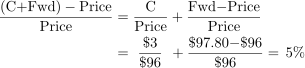
(6) $\begin{align*}\frac{(\mathrm{C} {+} \mathrm{Fwd}) - \mathrm{Price}}{\mathrm{Price}} &= \frac{\mathrm{C}}{\mathrm{Price}} + \frac{\mathrm{Fwd}{-} \mathrm{Price}}{\mathrm{Price}} \\ &= \,\,\frac{\mathdollar 3}{\mathdollar 96}\,\; + \frac{\mathdollar 97.80 {-} \mathdollar 96}{\mathdollar 96} = \, 5\%\end{align*}$

If the forward price turns out to match the realized future price on the nose, then the total payout from owning the bond next year would be $\mathdollar 100.80$ . Collect the $\mathdollar 3$ coupon and sell the bond for $\mathdollar 97.80$ . The $\mathdollar 3$ coupon amounts to a $3.13\%$ yield. The $\mathdollar 1.80$ price increase contributes an extra $1.87\%$ . The two components sum to deliver $r = 3.13\% + 1.87\% = 5\%$ .

The one-year-ahead forward price is not someone’s idle musings. It is a price forecast that bond traders arrive at with money at stake. A trader who’s convinced that the bond will sell for more than $\mathrm{Fwd} = \mathdollar 97.80$ next year can buy the forward and wait. A trader who believes that the future price will be lower can do the opposite. Every disagreement is an order, and orders move the quote. There’s no counterpart for SPY. Sure, analysts regularly set one-year-ahead price targets. But different analysts publish different numbers, and there’s no way to arbitrage the discrepancy in their views. You can’t buy or sell an SPY price target.

The bond market’s accuracy

A bond’s forward price is the market’s working prediction of the bond’s price a year in the future, $\mathrm{Fwd}_t \approx \mathbb{E}_t[\mathrm{Price}_{t+1}]$ . Nothing riskless holds the realized price to this prediction. A trader convinced that $\mathrm{Price}_{t+1}$ will come in above $\mathrm{Fwd}_t$ can buy the forward and wait, but waiting entails risk. Rates can move against him before the year is out. So the gap between the forward price and the realized price is a bet, not an arbitrage. The market cannot squeeze it to zero. It can only keep it small. How small? The prediction could be amazingly accurate, or it could be incredibly noisy. To find out, we just need to compare the traded forward price at time $t$ to the bond’s price level a year later. A simple first pass might look at

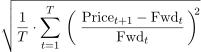
(7) $\begin{equation*}\sqrt{\frac{1}{T} \cdot \sum_{t=1}^T \, \bigg(\;\frac{\mathrm{Price}_{t+1} - \mathrm{Fwd}_t}{\mathrm{Fwd}_t}\,\bigg)^{\!\!2}}\end{equation*}$

If the output is $1\%$ , then it’d indicate that the realized bond price a year from now is usually ${\pm}1\%$ away from bond traders’ best guess today.

Here’s where the second feature of Treasury markets comes in. If we had run this exercise in equity markets, then there could be two reasons why next year’s price might have shifted: change in next year’s dividend forecast or change in the cap rate. As discussed above, the second channel is more impactful. But the first channel still exists when looking at equities. By contrast, it is completely absent in the Treasury market where a bond’s cash flows are known at the time of purchase. One year from now, our bond will be a 1-year bond with a single remaining payment of $\mathrm{C} + \mathrm{FV} = \mathdollar 103$ . Its price will be that $\mathdollar 103$ discounted at whatever the 1-year rate turns out to be. Every ingredient of $\mathrm{Price}_{t+1}$ except the rate is fixed in advance. So when the realized price misses the forward, there is exactly one suspect: the discount rate moved. And the conversion is one-for-one at this horizon, since the remaining claim has a duration of one year: a $\mathdollar 0.50$ price miss is a ${\sim}50\mathrm{bps}$ rate miss. Treasury forward-price errors are estimates of the noise in $r$ , in exactly the units we need, with nothing else mixed in.

When you look at real-world data, how noisy is the bond market’s best guess? Fed-fund futures are forwards written on the overnight rate a few months out. Betting against them has earned ${\sim}50\mathrm{bp}$ per year on average from 1988 to 2003 (Piazzesi and Swanson, 2008). At longer maturities, the errors arrive in price units, so it’s necessary to adjust the formula above to account for duration. A bond’s price miss is roughly its duration times its rate miss. Two-year notes miss by about ${\sim}2\%$ a year, which implies the rate is off by ${\pm}100\mathrm{bp}$ . Ten-year notes miss by ${\sim}6\%$ . With a duration of $8$ years, this pricing error translates to rate mistakes of ${\pm}75\mathrm{bp}$ . The long bond misses by ${\sim}10\%$ , which translates to rate noise of ${\pm}65\mathrm{bp}$ when assuming a duration of $18$ years. Every point on the curve tells the same story. The bond market’s best forecast of a rate is accurate to within $50\mathrm{bp}$ to $100\mathrm{bp}$ .

Equity traders would be thrilled if they could pin down SPY’s cap rate to the same level of precision. Treasuries generate the most accurate estimates for an asset’s discount rate. It is a number the assembled market backed by real money, and anyone holding a better estimate could have traded it into the quote. The errors are pure, because known cash flows leave the rate as the only moving part. Whatever noise survives under these conditions is noise that no investor, anywhere, could have forecasted away.

What it means for SPY

SPY’s cap rate is the same kind of object as the yield on a Treasury bond. It is the rate that turns a stream of future payments into today’s price. Noise in $(r{-}g)$ means the index’s price is wandering off its present-value path, exactly as a bond price wanders off its forward path when the rate moves. The bond market’s best rate forecasts miss by somewhere between $50\mathrm{bp}$ and $100\mathrm{bp}$ in a typical year. Take this result seriously and it becomes a precision limit for equity pricing.

The Gordon model says to capitalize SPY’s $\mathdollar 7.70/\mathrm{sh}$ NTM dividend forecast using a $100{\times}$ multiple. Above, we saw that the same factor of $100{\times}$ also magnifies cap-rate errors when calculating the percentage price impact. If equity investors cannot hope to estimate SPY’s cap rate to an accuracy better than ${\pm}50\mathrm{bp}$ , then the Gordon price can only be accurate to within

(8) $\begin{equation*}100 \times 0.5\% = {\pm}50\%\end{equation*}$

When using $(r{-}g)=1\%$ , the Gordon model says SPY should trade at $\mathdollar 7.70/\mathrm{sh} \times \big( \frac{1}{1\%} \big) = \mathdollar 770/\mathrm{sh}$ . If the correct cap rate could be as high as $1.5\%$ or as low as $0.5\%$ , then the true valuation could be anywhere from $\mathdollar 513/\mathrm{sh}$ to $\mathdollar 1{,}540/\mathrm{sh}$ , a range of more than $\mathdollar 1{,}000$ .

This is Fisher Black’s quip about how prices are “correct” to “within a factor of 2”. When using the canonical present-value model, the best achievable estimate of SPY’s cap rate leaves its price level undetermined to within $100 \times 0.5\% \approx 50\%$ . This is not a prediction of stock-market volatility. It is the size of the price fluctuations that could be explained by the unavoidable noise in the market’s best estimate of $(r{-}g)$ . No one knows SPY’s cap rate to an accuracy of ${\pm}50\mathrm{bp}$ . To really drive this point home, note that while SPY currently has a dividend yield of $1\%$ , its long-run average dividend yield is closer to $2\%$ . Many academic papers rely on this higher value for calibrations. This is a disagreement of ${+}100\mathrm{bp}$ .

Excess volatility puzzle

The above calculations put an entirely different spin on Shiller’s classic result. In his 1981 paper, he calculated the price implied by the S&P 500’s realized future dividend stream using a constant annual discount rate. He then compared this DDM-implied valuation to the index’s actual price level at the time. Figure 1 in the paper shows that the two time series are wildly different. The S&P 500’s realized price is $10{\times}$ more volatile than the implied price. The index’s dividend is extremely stable while its returns fluctuate by ${\pm}20\%$ from year to year.

Shiller (1981) studies a model in which investors (a) set price equal to expected discounted payoff, (b) have perfect foresight about those future payoffs, and (c) use a constant discount rate. This model clearly does not fit the level of the S&P 500. How did researchers respond to this finding? Well, they didn’t abandon assumption (a). Instead, they tried to generate additional return volatility by allowing for biased beliefs and letting the discount rate vary over time. e.g., in the late 1980s, Campbell and Shiller produced a dynamic extension of the Gordon model, which allowed $r$ and $g$ to vary over time. It is widely believed that this log-linear approximation to Gordon holds under arbitrary subjective beliefs.

But if you’re unwilling to abandon present-value logic, then this gets the story exactly backwards. Shiller calculated a DDM-implied price for the S&P 500 in an extremely simple way

(9) $\begin{equation*}\text{Implied Price}_t = \sum_{h=1}^{T-t} \frac{\mathrm{Div}_{t+h}}{(1{+}r)^h} \; + \; \frac{\overline{\text{Price}}}{(1{+}r)^{T-t}}\end{equation*}$

$T=1979$ is the last year in the sample. $\overline{\mathrm{Price}}$ is the S&P 500’s average detrended real price level during the sample period. This is not the theoretically correct thing to do. It parks every dividend payment beyond the sample in a single assumed terminal value. It uses the S&P 500’s realized future dividend payments rather than investors’ expectations of these payoffs. The correct discount rate need not be constant.

While not exactly pristine, suppose you think that Shiller’s implied price is roughly correct. Morally speaking, the formula above is clearly a present-value calculation. If you think the outcome of this formula is in the right ballpark, then the question is not: Why is the market price so volatile? The question is: How are market participants keeping the price level so damn close? Suppose the implied price were constant. In that case, an annual return volatility of $20\%$ would require knowing the S&P 500’s cap rate to within ${\pm}20\mathrm{bp}$ . This level of precision is far below anything observed even in bond markets.

If the bond market cannot pin down next year’s rate to better than ${\pm}50\mathrm{bp}$ , then how on earth are equity investors pricing the S&P 500 in a way that requires knowledge of $(r{-}g)$ to within ${\pm}20\mathrm{bp}$ ? If equity investors know SPY’s cap rate to within ${\pm}50\mathrm{bp}$ , then the correct valuation could be anywhere from $\mathdollar 7.70/\mathrm{sh} \times \big( \frac{1}{0.5\%} \big) \approx \mathdollar 1{,}540/\mathrm{sh}$ to $\mathdollar 7.70/\mathrm{sh} \times \big( \frac{1}{1.5\%} \big) \approx \mathdollar 513/\mathrm{sh}$ , a span of over $\mathdollar 1{,}000$ . With a precision of ${\pm}20\mathrm{bp}$ , the range shrinks to $\mathdollar 320$ : $\mathdollar 7.70/\mathrm{sh} \times \big( \frac{1}{0.8\%} \big) \approx \mathdollar 962/\mathrm{sh}$ to $\mathdollar 7.70/\mathrm{sh} \times \big( \frac{1}{1.2\%} \big) \approx \mathdollar 642/\mathrm{sh}$ . This massive improvement in accuracy is hard to fathom on present-value grounds.

Your Honor! I object…

You might balk at me calling the forward-price gap “noise.” Academics usually call it a time-varying risk premium. Fine. Call it whatever you want. Changing the name won’t supply the missing precision. If government bonds carry a risk premium that moves by ${\pm}50\mathrm{bp}$ from year to year, then the S&P 500 should carry a risk premium that moves by at least as much. Stocks are riskier than Treasuries. The return-predictability literature exists because expected equity returns are supposed to swing by percentage points across cycles, not basis points. A cap rate move of ${\pm}50\mathrm{bp}$ implies a price swing of ${\pm}50\%$ . We observe ${\pm}20\%$ . If you want to fly the “risk premium” banner, then you’d have to explain why the discount rate on the riskiest major asset class moves less than half as much as the discount rate on its safest one?

The remaining escape is to argue that $r$ and $g$ move together in a way that cancels out of the difference $(r{-}g)$ . But think about what this would require. The wandering in $\mathrm{d}r$ is observed: the risk-free leg alone moves by $50\mathrm{bp}$ or more in a typical year. So for the difference to stay pinned to within ${\pm}20\mathrm{bp}$ , you would need $\mathrm{d}g$ to shadow $\mathrm{d}r$ nearly move for move. Run the variance arithmetic: the growth forecast needs a spread between roughly $30\mathrm{bp}$ and $70\mathrm{bp}$ with a correlation to $\mathrm{d}r$ above $0.9$ , year after year, decade after decade. Measured long-run growth expectations show nothing like that co-movement with rates. That is not an assumption. It is a century of coincidences stacked one on top of the other.