Deriving the Gordon Model

The Gordon model is a mainstay of MBA classes and motivating examples. The model says that a stock’s current share price will equal its expected dividend next year, $\mathbb{E}_t[\text{Div}_{t+1}]$ , times a forward multiple, $\big( \frac{1}{\mathrm{r} - \mathrm{g}}\big)$ ,

(1) $\begin{equation*}\text{Price}_t = \mathbb{E}_t[\text{Div}_{t+1}] \times \bigg( \frac{1}{\mathrm{r} {-} \mathrm{g}}\bigg)\end{equation*}$

$\mathrm{r}$ is the stock’s annual risk-adjusted discount rate. A dollar paid out $4$ years from now is worth $\frac{\mathdollar 1}{(1+\mathrm{r})^4}$ today. $\mathrm{g} = \big(\frac{\mathbb{E}_t[\text{Div}_{t+h}]}{\text{Div}_t}\big)^{1/h}{-}1$ is the company’s anticipated dividend-growth rate at every horizon $h \geq 1$ .

Myron Gordon’s idea was to scale up next period’s dividend forecast by a factor of $\big( \frac{1}{\mathrm{r}-\mathrm{g}} \big)$ to capture the present value of the firm’s dividend stream from year $(t{+}2)$ onward. e.g., suppose a firm has promised to pay $\mathdollar 5.00/\mathrm{sh}$ in dividends next year. If investors apply a $10\%$ discount rate and anticipate $5\%$ annual dividend growth, then the Gordon model would price the stock at $\mathdollar 5.00/\mathrm{sh} \times \big( \frac{1}{10\%-5\%} \big) = \mathdollar 100/\mathrm{sh}$ .

There’s nothing remotely complicated about this calculation. Researchers all learn the Gordon pricing formula the first week of their PhD program. We’re all very comfortable reasoning in these terms. So it’s easy to forget how much work goes into producing the result. There’s nothing simple or straightforward about it. The key step in the derivation of the Gordon model isn’t about assuming constant parameters. It’s getting rid of the unknown future resale price, which is only a problem when applying present-value logic to stocks.

This post walks through what it takes to derive the Gordon model. I use the Lean proof assistant to do a proper accounting of all the assumptions and steps involved.

Perpetuities

The Gordon model prices stocks by pretending they are bonds. To see the logic, it’s important to understand why it’s easier to apply present-value logic to fixed-income assets. Let’s start with the simplest one: a perpetuity. This is an asset that will pay the same annual coupon starting next year and continuing on until Kingdom come. The present value of this perpetual stream of coupon payments is

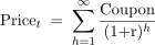
(2) $\begin{equation*}\text{Price}_t \;=\; \sum_{h=1}^{\infty} \frac{\text{Coupon}}{(1 {+} \mathrm{r})^h}\end{equation*}$

$\mathrm{r} > 0\%$ denotes the annual discount rate.

This geometric series can be simplified as follows

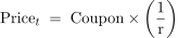
(3) $\begin{equation*}\text{Price}_t \;=\; \text{Coupon} \times \bigg( \frac{1}{\mathrm{r}} \bigg)\end{equation*}$

Doubling the annual coupon payment doubles the price of the perpetuity. Lowering the discount rate makes each dollar that a perpetuity delivers in the future more valuable today, thereby increasing the overall price.

Coupon Bonds

An $H$ -year coupon bond works like a perpetuity for the first $(H{-}1)$ years. Both pay the same coupon each year. However, in the final year $H$ , the coupon bond delivers its coupon payment as well as its face value, $\mathrm{FV}$ . The price of a coupon bond reflects the present value of its payout stream

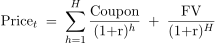
(4) $\begin{equation*}\text{Price}_t \;=\; \sum_{h=1}^{H} \frac{\text{Coupon}}{(1 {+} \mathrm{r})^h} \;+\; \frac{\mathrm{FV}}{(1{+}\mathrm{r})^H}\end{equation*}$

The present-value logic is the same. Only the payout stream has changed.

The face value determines the scale of the bond. The size of the coupon is typically reported as a fraction of this number, $\mathrm{Coupon} = \mathrm{c} \cdot \mathrm{FV}$ . Thus, we can write the price as

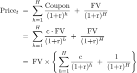
(5) $\begin{align*}\text{Price}_t \;&=\; \sum_{h=1}^{H} \frac{\text{Coupon}}{(1 {+} \mathrm{r})^h} \;+\; \frac{\mathrm{FV}}{(1{+}\mathrm{r})^H} \\ &=\; \sum_{h=1}^{H} \frac{\mathrm{c} \cdot \text{FV}}{(1 {+} \mathrm{r})^h} \;+\; \frac{\mathrm{FV}}{(1{+}\mathrm{r})^H} \\ &=\; \mathrm{FV} \times \Bigg\{ \sum_{h=1}^{H} \frac{\mathrm{c}\phantom{i}}{(1 {+} \mathrm{r})^h} \;+\; \frac{1\phantom{n}}{(1{+}\mathrm{r})^H} \Bigg\}\end{align*}$

The first term in the curly braces, $\sum_{h=1}^{H} \frac{\mathrm{c}\,}{(1 {+} \mathrm{r})^h}$ , is the present value of the coupons spun off by each dollar of face value. The second term, $\frac{1\phantom{n}}{(1{+}\mathrm{r})^H}$ , is the present value of receiving that dollar when the bond matures.

Par Value

The face value is the relevant reference point for pricing bonds. If $\text{Price}_t = \mathrm{FV}$ , then we say that a bond is “priced at par”. Each dollar of face value spins off a $\mathrm{c} \cdot \mathdollar 1$ coupon once a year for the next $H$ years. When priced at par, the present value of these coupons exactly offsets the loss from having to wait $H$ years to receive the dollar back

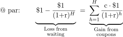
(6) $\begin{equation*}\text{@ par:} \qquad \underbrace{\phantom{\Bigg(}\!\!\!\!\mathdollar 1 - \frac{\mathdollar 1\phantom{m}}{(1{+}\mathrm{r})^H}}_{\substack{\text{Loss\phantom{j}from} \\ \text{waiting}}} \;=\; \underbrace{\sum_{h=1}^{H} \frac{\mathrm{c} \cdot \mathdollar 1}{(1 {+} \mathrm{r})^h}}_{\substack{\text{Gain\phantom{j}from} \\ \text{\phantom{t}coupons\phantom{t}}}}\end{equation*}$

These two forces offset when the coupon rate equals the discount rate, which is why par bonds have $\mathrm{c} = \mathrm{r}$ .

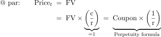
Bond traders use par pricing as a reference point when performing back-of-the-envelope calculations. When $\mathrm{Price}_t = \mathrm{FV}$ , it doesn’t matter whether you get paid the face value at time $(t{+}H)$ or continue to collect an infinite stream of coupons from year $([t{+}H]{+}1)$ onward

(7) $\begin{align*}\text{@ par:} \qquad \text{Price}_t \;&=\; \text{FV} \\ &=\; \text{FV} \times \underbrace{\bigg( \frac{\mathrm{c}}{\mathrm{r}} \bigg)}_{=1} \;=\; \underbrace{\text{Coupon} \times \bigg( \frac{1}{\mathrm{r}} \bigg)}_{\text{Perpetuity formula}}\end{align*}$

If $\mathrm{c} < \mathrm{r}$ , then the bond’s priced at a discount (below par). If $\mathrm{c} > \mathrm{r}$ , then it’s priced at a premium (above par).

Core Problem

At first glance, it seems like it should be possible to apply the same present-value logic to pricing stocks. The one-year-ahead pricing rule for stocks looks similar to the pricing formula for a one-year coupon bond

(8) $\begin{align*}\text{bond:} \qquad \text{Price}_t \;&=\; \frac{\;\;\!\mathrm{Coupon}\;\;\!}{1{+}\mathrm{r}} + \frac{\;\;\;\;\;\;\;\!\mathrm{FV}\;\;\;\;\;\;\;\!}{1 {+} \mathrm{r}} \\ \text{stock:} \qquad \text{Price}_t \;&=\; \frac{\mathbb{F}_t[\text{Div}_{t+1}]}{1{+}\mathrm{r}} + \frac{\mathbb{F}_t[\text{Price}_{t+1}]}{1 {+} \mathrm{r}}\end{align*}$

$\mathbb{F}_t[\cdot]$ denotes investors’ forecast given time- $t$ information. A forecast is just a number in investors’ heads. Nothing guarantees it obeys the laws of probability, so I reserve $\mathbb{E}_t[\cdot]$ for forecasts that do. This distinction will play a big role later on. Chekhov’s gun applies to both screenplays and academic research.

The stock’s forecasted dividend payment next year is kind of like the bond’s coupon. The stock’s anticipated resale price a year from now is sort of like the bond’s face value. However, there’s a key difference. For the bond, $\mathrm{Coupon}$ and $\mathrm{FV}$ are both known at the time of purchase. In ye olde times, when you bought a bond, you received a big piece of paper with a bunch of tabs on the bottom. Each year, you tore off a tab and mailed it in to receive your coupon. When the bond matured, you sent in the last tab and the big sheet of paper to get paid the face value. You couldn’t do this for a stock. Nobody knows $\mathrm{Div}_{t+1}$ or $\mathrm{Price}_{t+1}$ with certainty when you buy a share at time $t$ .

The core problem with using present-value logic to price equities is the forecasted resale price on the right-hand side, $\mathbb{F}_t[\mathrm{Price}_{t+1}]$ . If you’re trying to figure out the functional form of $\mathrm{Price}_t$ , then how are you supposed to know the right value to plug in for next year’s resale price? It is always possible to write an equation in which a stock’s current price equals the discounted payoff to owning a share next year. But for this equation to mean something, you need to remove the dependency of next year’s payoff on the future resale price. Otherwise, the relationship is circular.

Prior to Myron Gordon, people knew how to price bonds using present-value logic. But they didn’t know how to apply similar logic to assets like stocks where fluctuations in the future resale price represent a significant portion of the future payout. Gordon’s 1959 paper showed how to get around this problem by treating stocks like coupon bonds priced at par. Notice that the pricing rule is just a modified perpetuity formula, which includes an adjustment for a growing coupon. This is a bold claim about how stocks get priced. At the very least, it ain’t how people talk about pricing shares of Nvidia or Tesla.

Full Derivation

When researchers describe the Gordon model, they tend to focus on the fact that both $\mathrm{r}$ and $\mathrm{g}$ are constant. This is the least interesting part of the derivation. Let’s walk through what’s required to get from the one-period-ahead present-value formula to Myron Gordon’s result

(9) $\begin{equation*}\text{Price}_t \;=\; \frac{\mathbb{F}_t[\text{Div}_{t+1}] + \mathbb{F}_t[\text{Price}_{t+1}]}{1 + \mathrm{r}_t} \qquad \rightsquigarrow \qquad \text{Price}_t \;=\; \mathbb{E}_t[\mathrm{Div}_{t+1}] \times \bigg( \frac{1}{\mathrm{r}{-}\mathrm{g}} \bigg)\end{equation*}$

The discount rate now carries a time subscript. Nothing in one-period-ahead present-value logic requires investors to apply the same discount rate every year, so from here on I let $\mathrm{r}_t$ vary over time. There are 5 steps. The first 4 are where all the real heavy lifting takes place. $\mathrm{r}$ and $\mathrm{g}$ only lose their time subscripts in step #5 after the main formula has been derived. This is just cosmetic tidying-up.

Step #1: Assume Consistent Pricing

To iterate forward, investors must believe the one-period-ahead pricing rule holds at every future date $(t{+}h)$ . The same formula that governs today’s price must also govern the price targets in investors’ heads

(10) $\begin{equation*}\text{Price}_{t+h} = \frac{\mathbb{F}_{t+h}[\text{Div}_{(t+h)+1}] + \mathbb{F}_{t+h}[\text{Price}_{(t+h)+1}]}{1 + \mathrm{r}_{t+h}} \qquad \text{for all } h \geq 0\end{equation*}$

$\mathrm{r}_{t+h}$ is the one-period discount rate applied to payouts received at time $([t{+}h]{+}1)$ . i.e., each dollar paid the following year is worth $\frac{\mathdollar 1}{(1+\mathrm{r}_{t+h})}$ at time $(t{+}h)$ . One more assumption hides in this notation. Discount rates can differ across years, but the entire path $\mathrm{r}_t, \mathrm{r}_{t+1}, \mathrm{r}_{t+2}, \ldots$ is known at time $t$ .

There’s an important economic distinction between applying the formula today, $h{=}0$ , and applying the formula in future years, $h \geq 1$ . Even if most investors don’t think in present-value terms, you could argue that the invisible hand of the market somehow forces the current price to obey the one-period-ahead present-value rule at time $t$ . But you can’t make the same argument for $h \geq 1$ . The pricing formula for these future dates can only exist in investors’ heads. If they don’t think in present-value terms, then there’s no reason for the formula to hold. The claim is a substantive assumption about how investors think.

Step #2: Assume The Tower Property

The tower property says that today’s forecast of next year’s forecast is just today’s forecast

(11) $\begin{equation*}\mathbb{F}_t\big[\mathbb{F}_{t+1}[\,\cdot\,]\big] = \mathbb{F}_t[\,\cdot\,]\end{equation*}$

The same is true if we replace next year, $h{=}1$ , with any other longer horizon. Arbitrary forecasts do not have this feature. The tower property is only satisfied by conditional expectations that stem from a well-posed probability space. It is often referred to as the “law of iterated expectations”. I call it the “tower property” to emphasize the distinction between arbitrary forecasts and coherent expectations. From here on out, I write $\mathbb{E}_t[\cdot]$ rather than $\mathbb{F}_t[\cdot]$ .

One last thing. Coherent doesn’t mean correct. The law of iterated expectations can be applied to expectations that aren’t objectively correct. It’s a property of the belief structure, not whether these beliefs match the true data-generating process. Biased subjective expectations are a subset of all possible forms of incorrect beliefs. It’s possible to make incorrect forecasts that violate the laws of probability.

Step #3: Iterate Forward Finite Times

The next step is finite induction. Take the one-period-ahead pricing rule and replace the resale price on the right-hand side with its functional form for the following year. If you do this $(H{-}1)$ times, then you get the following expression

(12) $\begin{equation*}\text{Price}_t \;=\; \underbrace{\sum_{h=1}^{H} \frac{\mathbb{E}_t[\text{Div}_{t+h}]}{\prod_{k=0}^{h-1} (1 {+} \mathrm{r}_{t+k})}}_{\text{PV first H dividends}} \;+\; \underbrace{\frac{\mathbb{E}_t[\text{Price}_{t+H}]}{\prod_{k=0}^{H-1} (1 {+} \mathrm{r}_{t+k})}}_{\text{PV resale price}}\end{equation*}$

The company’s current share price reflects its expected discounted dividend payments over the next $H$ years plus the present value of the expected resale price $H$ years from now.

Notice that this step doesn’t purge the future resale price from the right-hand side. The date of reckoning has just been pushed farther into the future. In a sense, this makes the original problem worse. If next year’s resale price was hard to fathom, then why would investors have any idea about the price each share might sell for $20$ or $100$ years in the future? At this point, it’s not obvious progress has been made.

Step #4: Assume Limit Is Well-Behaved

The payoff to iterating forward only occurs when you take the infinite limit, $H \to \infty$ . We’re looking to remove the dependency of the current price on the expected future resale value. For this to happen, we need two things to be true:

Transversality. The expected discounted resale price must go to zero
(13) $\begin{equation*}\lim_{H \to \infty} \, \frac{\mathbb{E}_t[\text{Price}_{t+H}]}{\prod_{k=0}^{H-1} (1 {+} \mathrm{r}_{t+k})} \;=\; \mathdollar 0\end{equation*}$

The one-period recursion has infinitely many solutions. A rational bubble also satisfies it. Transversality selects the “correct” price, which reflects expected discounted dividends alone.
Convergence. The infinite sum of the stock’s expected discounted dividends must converge to a single finite number, and the answer cannot depend on the order in which the terms get added up. This second requirement is where the bite is. Adding up the discounted dividends in time order and getting a finite limit follows for free from step #3 plus transversality. Absolute convergence does not. Researchers often focus on transversality and take this second condition for granted. But both are strong assumptions. Convergence is a genuine premise of its own, not merely a footnote.

By making both assumptions, it’s possible to eliminate the future resale price entirely. The resulting pricing rule is known as the Dividend Discount Model (DDM). It says that a company’s share price at time $t$ should reflect the discounted value of its expected future dividend stream from time $(t{+}1)$ onward

(14) $\begin{equation*}\text{Price}_t \;=\; \sum_{h=1}^{\infty} \frac{\mathbb{E}_t[\text{Div}_{t+h}]}{\prod_{k=0}^{h-1} (1 {+} \mathrm{r}_{t+k})}\end{equation*}$

We’ve now overcome the main challenge in deriving a present-value pricing rule for stocks.

Step #5: Assume Constant Parameters

All the heavy lifting is already done. This last step is about ease-of-use. Most people don’t have clear views about a company’s likely dividend in 2077. They don’t have nuanced views about whether to apply a higher one-year discount rate in 2077 or 2076. So, to make the formula more practical, let’s assume that the stock’s future dividend grows at a constant annual rate

(15) $\begin{equation*}\mathbb{E}_t[\text{Div}_{t+h}] \;=\; (1 + \mathrm{g})^{h-1} \!\cdot \mathbb{E}_t[\text{Div}_{t+1}] \;=\; (1 + \mathrm{g})^h \cdot \text{Div}_t\end{equation*}$

Let’s also assume that the same annual discount rate gets applied to every horizon $h \geq 0$

(16) $\begin{equation*}{\textstyle \prod_{k=0}^{h-1}} (1 {+} \mathrm{r}_{t+k}) \;=\; (1 + \mathrm{r})^h\end{equation*}$

The assumption of constant parameters turns the infinite sum with a telescoping product in the denominator into a simple geometric series

(17) $\begin{align*}\text{Price}_t \;&=\; \sum_{h=1}^{\infty} \frac{\mathbb{E}_t[\text{Div}_{t+h}]}{\prod_{k=0}^{h-1} (1 {+} \mathrm{r}_{t+k})} \\ &=\; \sum_{h=1}^{\infty} \frac{(1{+}\mathrm{g})^{h-1} \cdot \mathbb{E}_t[\text{Div}_{t+1}]}{(1 {+} \mathrm{r})^h} \\ &=\; \mathbb{E}_t[\text{Div}_{t+1}] \times \sum_{h=1}^{\infty} \frac{(1{+}\mathrm{g})^{h-1}}{(1 {+} \mathrm{r})^{h\phantom{-1}}} \\ &=\; \mathbb{E}_t[\text{Div}_{t+1}] \times \bigg(\frac{1}{\mathrm{r} {-} \mathrm{g}}\bigg)\end{align*}$

Assuming constant $\mathrm{r}$ and $\mathrm{g}$ makes it possible to express the implications of the DDM in a clean way.

With constant parameters, the transversality and convergence assumptions in step #4 boil down to the requirement that $\mathrm{r} > \mathrm{g}$ . If this condition is violated, $\mathrm{r} \leq \mathrm{g}$ , then the present value of the stock’s expected discounted dividend stream will be infinite. e.g., suppose a stock’s future payout stream gets discounted at $\mathrm{r}=3\%$ annually and the company paid a $\mathdollar 1.00/\mathrm{sh}$ dividend last year. If the firm’s dividend-growth rate is $\mathrm{g}=4\%$ , then next year investors expect $\mathbb{E}_t[\mathrm{Div}_{t+1}] = \mathdollar 1.04/\mathrm{sh}$ . Had the firm maintained the same dividend, this cash flow would only be worth $\mathdollar 0.97$ today. But they expect an extra $\mathdollar 0.04$ in dividends next year, and this is more than enough to make up for the valuation drag created by discounting.

Assumption Accounting

I use Lean to properly account for all the different assumptions used in the derivation of the Gordon model. The hard part is getting rid of the price forecast on the right-hand side:

Assume that the one-period-ahead pricing rule holds today as well as at every future date. It governs observed prices and the price forecasts in investors’ heads.
Assume that investors’ price forecasts satisfy the tower property. This requires their subjective beliefs to represent conditional expectations that stem from a well-defined subjective probability measure.
Iterate forward a finite number of times, pushing the unknown future resale price far into the future.
Assume that the infinite limit has the properties needed to eliminate the current price’s dependence on the future resale price. These are transversality (a.k.a., no bubbles) and convergence.

The final step is purely cosmetic. It occurs after the troublesome resale price has already been expunged.

Assume constant $\mathrm{r}$ and $\mathrm{g}$ .

The standard telling treats step #5 as the key assumption behind the Gordon model, but the honest ledger shows it is the last and lightest. The core derivation lives in steps #1-4. In addition to maintaining the ledger, the proof in Lean shows that each of the load-bearing assumptions in these steps is necessary: the tower property, transversality, and convergence. There are explicit counterexamples that satisfy everything else and yet break the conclusion.

The point of running the Gordon model through a proof assistant is not the machinery. Every well-trained economist has seen all these ideas before. The issue is that researchers have gotten so familiar with Gordon logic that they often forget all that it requires. The derivation is neither short nor innocent. Lean forces you to reckon with every required step in the proof.