Public companies are not obligated to return all available cash to shareholders at the end of the year. When you buy a share of stock, you receive the portion of the firm’s free cash flow that it decides to distribute as dividends. Textbook finance theory assumes that shareholders focus on these future payoffs when pricing a stock. Asset-pricing theory all stems from one simple concept: price equals expected discounted payoff. This is a foundational principle behind every model.
The “cash flows” in the classic discounted cash-flow (DCF) model refer to the money paid to investors, not the money received by the company. The Gordon model says to value a stock by scaling up next year’s per-share dividend forecast to capture the value of all subsequent dividend payments
(1) ![\begin{equation*}\text{Gordon Valuation} = \sum_{h=1}^{\infty} \frac{\mathbb{F}[\mathrm{DPS}_h]}{(1{+}r)^h} = \mathbb{F}[\mathrm{DPS}_1] \times \bigg( \frac{1}{r - g} \bigg) \end{equation*}](https://alexchinco.com/wp-content/ql-cache/quicklatex.com-7da7943d17e20d34e3c31d02b7cf096e_l3.svg "Rendered by QuickLaTeX.com")
![\mathbb{F}[\mathrm{DPS}_h]](https://alexchinco.com/wp-content/ql-cache/quicklatex.com-39f22c15ddbadd7a1b6a2942014a86eb_l3.svg "Rendered by QuickLaTeX.com") is the forecasted dividend per share in
is the forecasted dividend per share in  years, and
  is the discount rate applied to these future payoffs, which are predicted to grow the same amount every year in perpetuity,
 ![\mathbb{F}[\mathrm{DPS}_h] = (1{+}g)^h \times \mathrm{DPS}](https://alexchinco.com/wp-content/ql-cache/quicklatex.com-470623fd87a6e54fb0d651ff3f234ea9_l3.svg "Rendered by QuickLaTeX.com") .
.
This may be how every academic model works, but it is not how sell-side analysts typically value a company. Most reports set a price target by capitalizing the firm’s predicted earnings at a reasonable recent multiple. The default valuation method is next year’s EPS (earnings per share) forecast times a trailing P/E. Instead of asking, “How much would the firm’s entire future dividend stream be worth in today’s dollars?”, analysts ask, “If the company were to announce next year’s predicted EPS today, how would it be valued given current market pricing?” Only around  of sell-side reports pay lip service to DCF analysis.
Roughly  in
in  reports includes a full-blown DCF model. This post examines how analysts actually implement DCF analysis in these reports. How do they arrive at a per-share equity valuation for a particular company? It turns out that the procedure looks very different from what most researchers have in mind. Analysts are not just plugging
  key numbers into Equation (1). The standard DCF playbook is connected to the Gordon model, but it isn’t approximately Gordon in a way that’s captured by time-varying parameters. The protocol deviates from textbook theory in fundamental ways. My point is not that analysts are wrong. My point is that they’re doing something much more interesting than most researchers currently appreciate.
Standard Playbook
Analysts do not use DCF to compute a company’s share price directly. Instead, the approach gets used to estimate the enterprise value (EV) of the entire firm as a whole. Analysts forecast the company’s free cash flow (FCFF) for the next few years and discount these anticipated cash flows at a weighted average cost of capital (WACC). Then they tack on a terminal value (TV), reflecting the present discounted value of all subsequent free cash flows. The combined expression looks something like this
(2) ![\begin{equation*}\mathrm{EV} = \sum_{h=1}^{H} \frac{\mathbb{F}[\mathrm{FCFF}_h]}{(1 {+} r)^h} + \frac{\mathrm{TV}}{(1 {+} r)^H} \end{equation*}](https://alexchinco.com/wp-content/ql-cache/quicklatex.com-382f94038d3206193054787e765403dc_l3.svg "Rendered by QuickLaTeX.com")
![\mathbb{F}[\mathrm{FCFF}_h]](https://alexchinco.com/wp-content/ql-cache/quicklatex.com-cd5ff78abac5611826980d9a25d3840a_l3.svg "Rendered by QuickLaTeX.com") denotes the firm’s forecasted FCFF years from now.
denotes the firm’s forecasted FCFF years from now.  denotes the length of the firm’s transitionary period. During this time, the company’s FCFF is assumed to grow at a faster rate, settling down at a lower sustainable growth rate from year
  onward.
After arriving at an enterprise value, the analyst then uses a bridge to convert the number into a per-share equity valuation. First, they deduct the book value of net debt. Then, they divide the result by the company’s current share count. The fair value is thus
(3) 
 is the difference between a company’s outstanding debt and its cash holdings.
Running Example
To fix ideas, I’ll be using a running example involving a company in the midst of a transformation. Over the next  years, the company’s FCFF is expected to grow quickly:
 ![\mathbb{F}[\mathrm{FCFF}_1] = \mathdollar 8\mathrm{M}](https://alexchinco.com/wp-content/ql-cache/quicklatex.com-455702dbf048446ebb3bd986b991e5f0_l3.svg "Rendered by QuickLaTeX.com") ,
, ![\mathbb{F}[\mathrm{FCFF}_2] = \mathdollar 12\mathrm{M}](https://alexchinco.com/wp-content/ql-cache/quicklatex.com-9f4de464fafa73a2b7bb5123a9a09245_l3.svg "Rendered by QuickLaTeX.com") ,
, ![\mathbb{F}[\mathrm{FCFF}_3] = \mathdollar 16\mathrm{M}](https://alexchinco.com/wp-content/ql-cache/quicklatex.com-8e1a55d08070f7ca4baeea296e91c906_l3.svg "Rendered by QuickLaTeX.com") , and
, and ![\mathbb{F}[\mathrm{FCFF}_4] = \mathdollar 20\mathrm{M}](https://alexchinco.com/wp-content/ql-cache/quicklatex.com-94f5aecfb54106d0affacb517bead6bf_l3.svg "Rendered by QuickLaTeX.com") . These forecasts give the company a -year compound annual growth rate (CAGR) of
. These forecasts give the company a -year compound annual growth rate (CAGR) of  . From year
  onward, the firm’s FCFF will grow at a more modest rate,
  . The firm has
  shares outstanding, and each share is priced at
  , giving the firm a market cap of
  . Assume a cost of equity of
  .
.
Yesterday, the company issued a -year coupon bond with a face value of  and a
and a  annual coupon rate. The bond was issued at par. Unfortunately for the firm, the yield on this bond jumped to
  this morning, causing the price to drop by roughly
  to
to  . Since the bond was issued at par, the firm’s balance sheet carries it at because GAAP does not mark debt to market. The firm holds
  in cash. Net debt at book is
  . Net debt at market would be
  . The firm faces a
  effective tax rate.
The Discount Rate
Analysts usually pick a discount rate equal to the firm’s weighted average cost of capital (WACC). It is the average tax-adjusted return on the firm’s capital
(4) 
Note that the  and
and  numbers in the WACC formula denote current market pricing, not book value at issuance. An unlevered firm will have a WACC equal to its cost of equity,
  . A highly leveraged firm will get discounted at a rate closer to its tax-adjusted cost of debt,
  , which will be lower.
Plugging in numbers, the firm in our running example would face an annual discount rate of
(5) 
The company’s  leverage ratio closes
  of the gap between
  and
and  . Debt gets discounted at rather than
  because interest payments don’t face a tax.
The Terminal Value
During the next couple of years, the firm is growing quickly. The terminal-value term in Equation (2),  , reflects the present value of the company’s subsequent FCFF stream after this transitionary period has ended. It is usually computed with either a perpetuity or with a trailing/comps multiple
(6) ![\begin{equation*}\mathrm{TV} = \mathbb{F}[\mathrm{FCFF}_{H+1}] \times \begin{cases} \big( \tfrac{1}{r - g}\big) &\text{Gordon} \\ \mathrm{EV/FCFF} &\text{Comps} \end{cases}\end{equation*}](https://alexchinco.com/wp-content/ql-cache/quicklatex.com-3cbca3dce80390086eb46824589623de_l3.svg "Rendered by QuickLaTeX.com")
The first option assumes that the firm’s FCFF will grow at an annual rate of  from year onward. The second option uses the firm’s current EV/FCFF multiple or the average multiple for a set of comparable firms to capitalize the company’s anticipated FCF in year .
In our running example, the firm has a -year transitionary period in which its FCFF grows at per year. The analyst believes that its FCFF will grow from ![\mathbb{F}[\mathrm{FCFF}_1]=\mathdollar 8\mathrm{M}](https://alexchinco.com/wp-content/ql-cache/quicklatex.com-ca2cc8c8660368cf7cb4766f8f13d708_l3.svg "Rendered by QuickLaTeX.com") next year to
next year to ![\mathbb{F}[\mathrm{FCFF}_4]=\mathdollar 20\mathrm{M}](https://alexchinco.com/wp-content/ql-cache/quicklatex.com-0f0538ddb89d94345929f2ea0a5ea284_l3.svg "Rendered by QuickLaTeX.com") in year
in year  . After that, the company’s FCFF stream will grow at
  per year in perpetuity. This lower more-sustainable growth rate puts the firm’s forecast for year
  at
at
(7) ![\begin{equation*}\mathbb{F}[\mathrm{FCFF}_5] = (1{+}3\%)\times \mathdollar 20\mathrm{M} = \mathdollar 20.6\mathrm{M}\end{equation*}](https://alexchinco.com/wp-content/ql-cache/quicklatex.com-6d108c92d7845e36b79dbc9cb0993bf0_l3.svg "Rendered by QuickLaTeX.com")
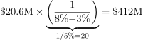
The firm’s  WACC and
  growth rate give it a cap rate of
  . At a terminal multiple of
  , the company’s terminal value would be
(8) 
Discounting this terminal value back years at  gives
gives 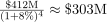 .
.
All Together Now
Here’s how all the pieces come together in the running example. The table below shows the company’s predicted FCFF stream over the next years as well as its terminal value
![\begin{equation*}\begin{array}{r|ccccc} \text{Horizon, } h & 1 & 2 & 3 & 4 & \mathrm{TV} \\ \hline \mathbb{F}[\mathrm{FCFF}_h] & \mathdollar 8.0\mathrm{M} & \mathdollar 12.0\mathrm{M} & \mathdollar 16.0\mathrm{M} & \mathdollar 20.0\mathrm{M} & \mathdollar 412.0\mathrm{M} \\ \frac{\mathbb{F}[\mathrm{FCFF}_h]}{(1+8\%)^h} & \mathdollar 7.4\mathrm{M} & \mathdollar 10.3\mathrm{M} & \mathdollar 12.7\mathrm{M} & \mathdollar 14.7\mathrm{M} & \mathdollar 302.8\mathrm{M} \end{array}\end{equation*}](https://alexchinco.com/wp-content/ql-cache/quicklatex.com-c3c7341a1007570f5dce8a9f6723d09e_l3.svg "Rendered by QuickLaTeX.com")
Combined, the firm’s first years of FCFF are worth  in today’s dollars. After discounting, its terminal value is worth
  . Together, these two components produce a total enterprise value of
  , with roughly
  coming at the end.
An analyst would now need to convert this  enterprise value into a per-share equity valuation. They do this using a bridge. The first step involves deducting the book value of the firm’s net debt,
  . The resulting difference is meant to capture the combined value of shareholders’ equity stake. To get a per-share number, the analyst then divides by the company’s current share count
(9) 
The company in our running example is trading at , so this implies  upside.
FCFF, Not Payoffs
Now that we understand what analysts do, let’s talk about the ways that it differs from what researchers assume. First and foremost, the standard DCF implementation capitalizes the cash the firm could pay rather than the cash the firm will pay. The resulting share price doesn’t reflect the discounted payoff stream that investors expect to receive. Analysts use a DCF model to capitalize money received by the firm, not money paid to investors. Every textbook model takes it for granted that investor payoffs and corporate proceeds are the same thing. If that’s the case, then the way that analysts implement DCF analysis isn’t inconsistent with standard theory.
The decision to focus on FCFF is particularly noteworthy. The line item represents the maximum dividend that an unlevered firm could distribute to its shareholders, not the dividend payment shareholders actually receive. The firm in our running example will produce  of FCFF next year. The company has promised
  to bondholders. After adjusting for taxes, this leaves
  . The firm can use this money to distribute a dividend, buy back shares, pay down its existing debt, acquire another firm, or add to its cash balance. In principle, shareholders might not receive any of these funds. For Equations (1) and (3) to be equivalent, a firm would have to invest any money not paid to *current stakeholders* at exactly .
Every report that builds a DCF model could have calculated the total payout to all stakeholders. The enterprise-level analog to dividend payments would be
(10) 
All you need to do is take FCFF and subtract off the tax adjusted interest payment and any increase in cash. The resulting amount of money must have been paid to current shareholders (dividends or buybacks), the firm’s creditors (debt paydown), or outside shareholders (acquisitions). Nobody does this.
Transition Period
Roughly of sell-side reports include a full-fledged DCF model. Almost all of these reports include a transition period with higher FCFF growth. When researchers think about a DCF model, they usually picture some version of the Gordon pricing rule in Equation (1). But the vast majority of DCF models that analysts write down do not assume sustainable long-term growth right away.  out of reports that include a detailed DCF analysis set
  . The analyst assumes the existence of an initial transition period in which the firm will grow at a much faster rate than .
In the running example, the transition lasts years. Think about what would happen if an analyst tried to remove this part of the model. First, suppose the analyst tried to set  without changing any other inputs. In this case, the resulting enterprise value would be far too low. The company is only predicted to generate of FCFF next year. So, with and , the Gordon-implied valuation would be
(11) 
After subtracting off net debt of and dividing by shares, the analyst would arrive at a share price of  . The analyst can’t publish such a low number. The firm is currently trading at .
Maybe the analyst can fix the problem by discounting at a lower discount rate? Nope. This would require discounting FCFF at the firm’s cost of debt, . To get an enterprise value of , you’d need
(12) 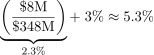
The implied multiple would also be absurdly high,  . Those are laughable numbers.
Thus, the requirement that puts analysts between a rock and a hard place. Allowing for provides a way out. A short-term runup makes it possible to quote a valuation of  without violating professional norms. The analyst gets to use a reasonable sounding WACC. They can point to a sensible
  multiple. All they have to do is argue that, before settling onto a more stable trajectory, the firm will initially grow at a faster
  clip for the next years.
Identification Problem
These transition periods create a serious identification problem for researchers looking to back out an analyst’s discount rate from IBES data. Those numbers contain an analyst’s forecast for next year (ignore the FCFF-vs-EPS distinction), their predicted long-term growth rate, and a price target. The choice of that justifies this price target depends on the analyst’s choice of transition dynamics. How long will the firm’s transition period last,  ? How fast will the firm grow during this time? Neither variable shows up in IBES.
To illustrate the severity of the problem, think about what the firm from the running example would look like in IBES. A researcher would see the analyst’s forecast for next year, , and the analyst’s long-term growth rate, . IBES might also contain a price target of . What IBES doesn’t tell you is the length of the analyst’s assumed transition period, , or the assumed CAGR during this period, . The table below shows how the implied changes as you adjust , holding fixed all observable quantities and setting 
![\begin{equation*}\begin{array}{r|rrrrr} H & 0 & 2 & 4 & 6 & 8 \\ \hline \mathbb{F}[\mathrm{FCFF}_{H+1}] & \mathdollar 8.0\mathrm{M} & \mathdollar 12.7\mathrm{M} & \mathdollar 20.6\mathrm{M} & \mathdollar 32.7\mathrm{M} & \mathdollar 51.9\mathrm{M} \\ \text{Implied }r & 5.3\% & 6.4\% & 8.0\% & 9.9\% & 11.9\% \end{array}\end{equation*}](https://alexchinco.com/wp-content/ql-cache/quicklatex.com-202ca84589a528684a681a7d99f257c3_l3.svg "Rendered by QuickLaTeX.com")
Without knowing how long the analyst assumed that the firm would grow , a researcher cannot tell whether  ,
,  , or
, or  . All these numbers are consistent with a valuation.
Required Precision
DCF analysis comes with a natural measuring stick for the size of the errors: the present value of the firm’s FCFF forecast for next year. In the running example, this is ![\frac{\mathbb{F}[\mathrm{FCFF}_1]}{1+r} = \frac{\mathdollar 8\mathrm{M}}{1+8\%} = \mathdollar 7.4\mathrm{M}](https://alexchinco.com/wp-content/ql-cache/quicklatex.com-47e99bc17e8e595d82cd99a1956f4b20_l3.svg "Rendered by QuickLaTeX.com") . If all you’re doing is adding up expected discounted cash flows, then it’d be a problem if you skipped or double-counted one. An error of
. If all you’re doing is adding up expected discounted cash flows, then it’d be a problem if you skipped or double-counted one. An error of  in enterprise value is the same as forgetting to count next year’s FCFF or including the number twice. Either way, a decision that alters enterprise value by
  is a big deal.
If the firm’s enterprise value fell to  , the company’s share price would fall by
  to
to
(13) 
That is a change of roughly  . So, anything that moves the company’s share price by more than
  is tantamount to forgetting to count a year of FCFF or double counting that year.
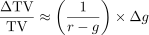
The terminal growth rate, , describes how a firm’s FCFF will grow in steady state. Forever is a long time. And, with so many years to worry about, small differences in an analyst’s choice of can compound into huge changes in the firm’s terminal value. The effect of a  change in the long-run growth rate will scale with the firm’s Gordon multiple
(14) 
The precision with which analysts quote tells you that they aren’t thinking along these lines. Most quote nice round numbers near  or .
or .
The firm in our running example has a cap rate of  , which implies that a
  increase in the terminal growth rate will cause the firm’s terminal value to rise by
(15) 
Apply that to the  present value of the terminal value in the running example.
  would move this number by roughly , an amount equal to the present value of next year’s anticipated FCFF. Yet, most reports quote in steps of
  , an increment half as precise as required by theory.
Market vs Book Value
The firm’s debt shows up in two different places in Equation (3): a) the WACC formula for the discount rate used to compute the firm’s EV; and b) the bridge used to translate this number into a share price. In the first case, the debt is taken at market value. In the second case, the book value of debt is used. For the firm in the running example, the bridge subtracts for a bond the firm could buy back for . That  gap understates the firm’s equity value by , resulting in a share price that is
  too low. The WACC is right. The bridge is wrong. Suppose that the firm’s credit rating deteriorates further so that its bond trades at
  , not . Market net debt would now be
  , but the bridge would still sit at . The firm’s equity value would now be understated by
  , which amounts to .
The analyst above calculated his WACC assuming a leverage of  . The equity value in the denominator comes from the fact that the company’s shares currently trade at and there are shares in circulation. However, this choice of WACC puts the value of each share at . At this price point, the firm’s equity value would be
  , not , and the firm’s leverage would be
  , not
, not  . The internally consistent calculation would produce a higher WACC,
  , because there is less debt and less shield. Iterating to this fixed point gives an enterprise value of
  and per-share valuation of
  . Nobody does that. Literally. No one. Analysts just ignore this fixed-point problem. The result is a rate that is
  too low and a share price that is overvalued by
  .
.
Why does a  move in the rate produce an move in the price? Start with a company that has no runup, just a perpetuity growing at . Its price is
  times
times  , so a change in the rate moves prices by
(16) 
The  company in the running example sees its enterprise value fall by
  in response to a
  increase in the rate. The firm’s enterprise value falls by
  , from to .
The extra of decline comes from the bridge. Net debt is a fixed , so the entire  drop in enterprise value is borne by shareholders
(17) 
Since equity only constitutes  of enterprise value, the bridge turns the
  decline in enterprise value into a
  drop in the share price.
Tax shield of interest
The firm in our running example has an WACC when including the tax shield of interest. Without the factor of  , the company’s discount rate would rise to
(18) 
At this higher rate, the firm’s anticipated FCFF path would be worth just  . In other words, the firm’s enterprise value contains a tax shield worth around
  .
.
The full  does not appear on the firm’s financial statements. Its balance sheet shows a single bond that will mature in year . The shield on that bond is
  a year for three years. This
  gap is roughly
  larger than the precision cutoff
(19) 
The difference will be even larger for newly distressed firms with high costs of debt. Discounting FCFF at a WACC is only exact when the firm continually rebalances its debt to a fixed share of value.
The Point Of DCF
Each section above describes a discrepancy. Each one vanishes under certain special conditions. Together, these conditions describe a particular kind of firm. For such a company, none of the issues outlined above would matter. Here’s what that company would look like:
- The firm must be investment grade. The company’s debt should trade at par. Its bonds ought to be issued recently or carry a floating rate. The firm’s credit rating should be AAA and never budge. Under these conditions, it won’t matter whether you use net debt at book or market value. Both are .
- The firm’s tax shield must be correctly valued. Its debt-to-EV ratio must remain constant. The company must refinance every bond at maturity. And it must have steady taxable income, so that every dollar of interest gets deducted. Under those conditions, the firm will collect the full shield implied by discounting FCFF at WACC.
- The analyst’s valuation must be close to the current market price. Otherwise the leverage ratio used to compute the WACC will not match the leverage ratio implied by the analyst’s own valuation, and the discount rate will be inconsistent with the number it produced. In practice, this means DCF confirms the market rather than disputes it.
- The firm must pay out nearly all available free cash flow each year or reinvest the money at the analyst’s WACC. If retained cash and acquisitions are either
 or NPV neutral, then discounting expected future FCFF is the same thing as discounting expected future payouts. In practice, only large dividend payers meet this condition. Growth-stock initiations never do.
 - The firm must have a clearly defined runup period, which everyone can agree upon. A massive production facility will come online in years. A new drug will get approved in years. It will take
 years for a merger to close. The company’s favorable current lease agreement will expire in years. The interim path is a schedule rather than a story, and the terminal year is the first normal year. Very few reports tie the runup to a dated event. The ones that do are hotel chains with an opening schedule that halves at stated dates, a device maker with an approval year, and Tesla with 2013 Model S volumes. Everywhere else the runup is a fade toward with nothing scheduled.
 - The firm’s terminal growth rate must be a credible forecast. The firm’s FCFF stream should grow with the economy after completing the runup phase. at nominal GDP growth must be a credible belief.
These statements describe a mature, investment-grade, fully-distributing firm going through one well-defined transition with a known end date. Think about a regulated utility completing a rate-base build. An oil-pipeline company with a contracted expansion coming online in a year or two. A stable industrial company that is midway through integrating a big recent acquisition.
Now notice what the DCF adds for such a firm. Once the transition ends, the firm trades like its peers. So the terminal multiple is a number the analyst could have looked up. and a peer EV/FCFF of are the same number doing the same job. Only one of them can be checked against a screen. That is why analysts so often close with a comp multiple rather than a Gordon multiple. The comp close is the analyst admitting that and were never the point.
The point of writing down a DCF model has nothing to do with the core logic behind the Gordon pricing rule in Equation (1). The only thing DCF analysis adds for this kind of firm is the runup. It answers one question: How long until this firm will look like its peers again? For a firm with a real transition, that answer is worth having. For a firm with no transition, there is no point to performing the DCF exercise. You might as well capitalize next year’s FCFF forecast at a reasonable recent multiple and be done with it.